VBA - Error Trapping

When an error occurs while executing the code, VBA treats that error as fatal and stops executing the code then and there, with an error alert message to the user. While at times this is what you may want, most of the times you will just have to continue running the code and do other jobs that macro was supposed to do. For this, we have to use what is called an Error Trapping. VBA provides ways to tackle with that error without interrupting the code. Let’s see what options we have to do that.

On Error Statement

This statement enables error-handling routine and you can specify from where the code should continue executing. We have 3 options to provide such location.

On Error Resume Next

This tells VBA to ignore the error and continue running the code from immediate next line of code following the line where the error occurred.

This error handler will be active through out your code. No matter how many times errors occurr in your procedure, VBA always executes the next line. But be careful, with this line, VBA ignores any kind of error. If you don’t take care, it may result into ignoring few errors that should not be ignored.

On Error GoTo line

This enables the error-handling routine to start at the line specified in the argument. The line argument is any line label or line number. The specified line must be in the same procedure as the On Error statement; otherwise, a compile-time error occurs.

Note that, on first occurrence of first error, VBA starts executing the code from line given as argument and continues executing the lines below it till the End Sub.

Once executed, error handler will be disabled for further use. That means, On Error GoTo statment can be used for only one error in a procedure.

On Error GoTo 0

Disables any error handler that is in the current procedure!

Let's see the error handling through an example. We will deliberately do something that causes an error. How about try to enter some value in a protected sheet and that will cause an error? Copy/Paste the below code to your module! Protect the active sheet. Click anywhere on the code in VBA and press F8 repeatedly to run the macro line by line. On each press of F8, you can notice where the focus is going.

Example –On Error Resume Next

Sub Test()
On Error Resume Next 'Defining the error trapping, on error focus should go to next line
ActiveCell.Value = 1000 'try to enter some random value in active cell
If Err.Number <> 0 Then 'check if error occurred?
    MsgBox ("Error Occurred") 'Yes? then message box saying so
Else
    MsgBox ("Done") 'No? Then all done.
End If
End Sub

Run this code by repeatedly pressing F8. Now you see that no matter what, focus will always go to the next line. We are trapping the error by If-Then-Else-End If statements.

Example –On Error Goto line

Sub Test()
On Error GoTo ErrorHandler 'Defining the error trapping, focus should go to a line named ErrorHandler below
ActiveCell.Value = 1000 'try to enter some random value in active cell
Exit Sub 'If no error, procedure should stop here

ErrorHandler: MsgBox ("Sorry, Error " & Err.Number & " Occurred") 'This line contains what to do in case of error
End Sub

If you noticed, from ActiveCell.Value = 1000 line, focus will change to ErrorHandler, as there will be an error when executing that line and we asked VBA to go to ErrorHandler on error occurrence. On one more press F8, a message box is shown informing the error number to the user.

Err Object

Wherever there is an error, VBA keeps that error information in Err object. You can use this information to know more about the type of error. You can in turn display the information to the user as we did in our earlier code. Err.Number provides the system assigned number of this error. There is also Err.Description will provide the description of the error. See other options available under Err object and explore.

VBA - If Then Else Endif

Do you remember the Excel built-in function IF? You can provide a condition to be evaluated by IF and provide a calculation / value if result is TRUE and provide a different calculation / value if result is FALSE. In similar lines, VBA also provides a feature i.e.. IF statement. Syntax for this is as below.

Form 1 – In One Line – Without Else Condition

If condition Then statement

If: is the key word to call this feature

Condition: what do you want to evaluate. You can give one or more conditions to evaluate (we will see how)

Statement: what if condition is met.

We are not defining what to do if condition is not met so macro will do nothing (moves to next available line of code).

Example: If ActiveCell.Value = 5 Then MsgBox(ActiveCell.Value)

This form is best used if you just want to evaluate one condition followed by single line action if condition is true. No action if condition is false.

Form 2 – In One Line - With Else Condition

If condition Then statement [Else elsestatement]

Other key words are similar as above form.

Elsestatement: What if condition is not met

Example: If ActiveCell.Value = 5 Then MsgBox(ActiveCell.Value) Else MsgBox(“No Match”)

This form is best used if you just want to evaluate one condition followed by single action if condition is true and a single line action if condition is false.

Form 3 – Multiple Lines - Without Else Condition

If condition Then

statement

Endif

Example:

If ActiveCell.Value = 5 Then
    MsgBox(ActiveCell.Value)
End If

Form 4 – Multiple Lines – With Else Condition

If condition Then

statement

Else

elsestatement

End If

Example:

If ActiveCell.Value = 5 Then
     MsgBox(ActiveCell.Value)
Else
     MsgBox(“No Match”)
End If

Form 5 – Multiple Lines - Multiple Else conditions

If condition Then
     statement
Elseif condition Then
     Elsestatement
Elseif condition Then
     Elsestatement
……………………….
Else
statement
End If

Example:

If ActiveCell.Value = 5 Then
      MsgBox(ActiveCell.Value)
Elseif ActiveCell.Value = 4 Then
      MsgBox(Application.UserName)
Elseif ActiveCell.Value = 3 Then
      MsgBox(“Welcome To The World”)
Else
      MsgBox(“Bye Guys”)
End If

Above examples are pretty much self explanatory. Copy them to a VBA module, enter a value in a cell and execute the macro. We will use many If Then Else statements in our forth coming macros. Stay tuned!!

Control The Cursor Movement on Pressing Enter

Typically, whenever you press Enter in Excel, cursor will move one box down (there are few exceptions, that’s not the point for this post). Few know that you can command Excel to behave differently upon pressing Enter viz. do nothing, go Up, Left or Right. Let’s see how to do that.

Excel 2010 and later:

No Cursor Movement after Enter

File tab > Options > Advanced tab > Editing options segment > clear the check box After pressing Enter, move selection > OK.

To Move Cursor In a Direction

File tab > Options > Advanced tab > Editing options segment > check the check box After pressing Enter, move selection > and select the direction you want the cursor to move in Direction drop down. Available options are Down, Right, Up and Left > OK.

Excel 2007:

No Cursor Movement after Enter

Click the Microsoft Office button > Excel Options > Advanced tab > Editing options segment > clear the check box After pressing Enter, move selection > OK.

To Move Cursor In a Direction

Click the Microsoft Office button > Excel Options > Advanced tab > Editing options segment > check the check box After pressing Enter, move selection > and select the direction you want the cursor to move in Direction drop down. Available options are Down, Right, Up and Left > OK.

Excel 2003:

No Cursor Movement after Enter

Tools menu > Options > Edit tab > clear the check box Move selection after Enter > OK.

To Move Cursor In a Direction

Tools menu > Options > Edit tab check the check box Move selection after Enter > and select the direction you want the cursor to move in Direction drop down. Available options are Down, Right, Up and Left > OK.

Once you are done with above steps, press Enter in excel and see how the cursor is moving.

Live Preview

Excel 2007 introduced a concept called Live Preview. Using this, you can view how the format change you are about to make actually look like, even before applying that change. This saves you the time you would otherwise spend on applying various formats and removing the applied format if you don’t like it.

You can access this feature by hovering the mouse over desired format options and wait a second, Excel will automatically update the selection to show how that will look like once the highlighted format applied. You just need to click on those options if you fancy or move away from it if you don’t like. That’s all.

Example:

To check different font sizes: Select the cells you want to change font size and Home tab > Font group > click the Font Size box down-arrow, and then move the pointer over different font sizes. Observe the cells you selected, they will change the size as you hover the mouse.

You can preview font formatting, quick styles, picture formatting using this feature. If you are using Excel 2010, you can also preview the Paste commands such as Keep Source Column Widths, No Borders, or Keep Source Formatting.

Though this option is awesome, if you feel that you don’t require live preview, there is an option to turn this feature off. Let’s see how.

Excel 2007:

Click the Microsoft Office button > Excel Options > Popular tab > Top options for working with Excel segment > clear the Enable Live Preview check box.

Excel 2010 and later:

File tab > Options > General > User Interface options segment > clear the Enable Live Preview check box.

Follow the same steps but check the box if you want to enable this feature.

Use Custom Number Formats Across Workbooks

We have been seeing about how to create custom data/time & number formats in a series of posts.  If you follow those codes carefully, by now you must be able to create formats as you require. There is a problem with these custom formats. They will be saved in the workbook you created them in and will not be available for other workbooks. If you spent an hour to create a custom number and want to use it across all Excel books anytime, you will have to save that workbook you have the customer format as a template.

Templates can contain the sheets, default text (such as page headers and column and row labels), formulas, macros, styles, and other formatting you want in all new workbooks you create.

Once you create a workbook with your custom format, save it as a template as below.

• Click on File tab > Save As (Excel 2010) / Microsoft Office Button > Save As (Excel 2007) / File menu > Save As (Excel 2003)
• Save as type box, click Excel Template or Excel 97-2003 Template (Excel 2007 or later) / Template (Excel 2003 or lower)
• Give any name you want to this workbook and click Save.

Next time onwards, whenever you want your custom formatting required in a new workbook, you will have to create a new workbook using File tab > New > New from existing (Excel 2010) / Microsoft Office Button > New > New from existing (Excel 2007) / File menu > New > From existing workbook(Excel 2003).

If you think this is too much to do or want your custom format available whenever you open Excel, you may want to save your template in XLStartup folder or alternate startup folder.

Custom Number Format - Examples

We have been seeing about different formatting available in Excel. In the last post, we saw about the codes used for custom number formats. Let’s see few examples now on how to use the code we learnt.

Display Whole Positive numbers ONLY

Yeah, weird, but I want it. I want to display the contents of the cells only if they are positive whole numbers like 1, 2, 3...and so on. Any others like negative numbers, text or decimals should not be shown in the cell. Let’s see how to code them.

I will break down our logic in parts.

• We want positive numbers to display but no decimals
• We don’t want to show negative numbers
• We don’t want to show zeros
• No text either

From what we learnt from the code in last post,

• Every cell can have 4 parts of display.
• If we don’t want a part to display, we can just enter a semi colon in that place.
• To display numbers we can use any one of 0, # and ? depending on your need. I will use 0.

Following the above logic, I can deduce the below code.

0;;;

Select a cell and apply above custom format. Enter different types of data in the cell and see how Excel will display or hide them.

Similarly you can code to show only negative numbers (use ;-0;;) note the minus sign before zero;, display zeros only (use ;;0;) and to display text only (;;;@). Needless to say, you can use combination of two or more criteria, such as show only positive and negative numbers and hide zeros & text (use 0;-0;;).

To display numbers with up to 2 decimals, you will replace 0 in above codes with 0.00 and so on based on your requirement.

Show Positive Numbers in Green, Negative in Red, Zeros in Blue and Text in Yellow

[Green]0;[Red]-0;[Blue]0;[Yellow]@

Display Nothing

;;;

Always Display X Number of Digits (Leading Zeros)

Bank account numbers for example will have fixed number of digits. Account numbers that doesn’t have those many digits will be prefixed with leading zeros. Like, if fixed length is 10 digits and you enter 12345, Excel can show it as 0000123545. If that is your need, you can use below code.

0000000000;;;

Above code should contain those many zeros as the number of digits you want. It is coded not to show negative, zeros & text.

Below is the picture showing how positive, negative, zeros & text appearing under different format codes as given above.

Display Telephone Number Style 1-800-333-3333

0-000-000-0000

Entering 1800333333 in this cell will show the number as 1-800-333-3333.

Display Numbers in Thousands / Millions

Round Off To Nearest Millions / Thousands / Numbers Based On the Number Entered

[>=1000000]0,, ;[>=1000]0, ;0

Above code displays values greater than or equal to 1 million rounded to nearest one million. If the entered number is not greater than or equal to 1 million, but is greater than or equal to 1000, then the value is rounded to nearest thousand. If neither condition is met then the figure will be displayed rounded to the nearest whole number.

Try different combinations in the code and explore it for yourself. Remember, you will learn excel better by doing trial and error yourself. But if you tried and couldn't get some format you needed, let me know. Happy Learning!!

Custom Number Format - Introduction

Note that formatting a number will ONLY change the appearance of it. That is, how you see the number on the screen changes but actual number you enter is NOT changed. We already saw how to build custom date & time format. So we are familiar with codes that represent the data.

A number format is coded in 4 parts. Each part of the code represents display format for positive numbers, negative numbers, zero values, and text respectively. Each of the part is separated by a semicolon (;). Syntax of this format is as below.

<POSITIVE>;<NEGATIVE>;<ZERO>;<TEXT>

You needn't write code for all 4 parts of the number. Excel has defaults and it can manage without coding few parts specifically. Let’s see what rules apply here.

• If you enter one code section – Excel take it for all the numbers (same format for positive, negative & zeros), default formatting for text
• If you enter two sections – First part is considered for positive numbers & zeros, second part is for negative numbers. Default formatting for text
• If you enter three sections – First part is considered for positive numbers, second part is for negative numbers, third for zeros. Default formatting for text
• If you want to skip a particular section, you place a semicolon for that section.

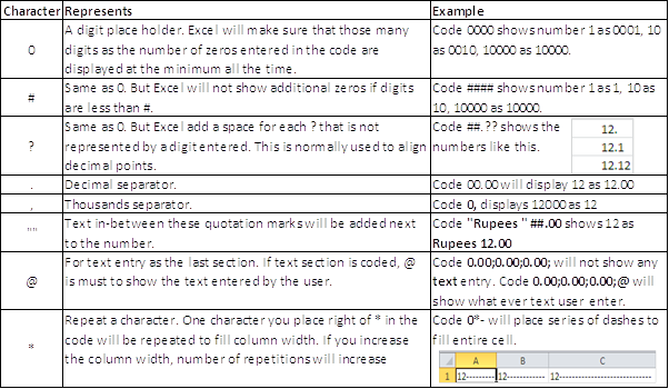
Do you remember the date & time formats we saw already? Excel provides few characters to represent each unit. For example: alphabet d represents date, m for month etc. In the same way, Excel has few representative characters to denote numbers. See the table below.

Note:

• If you enter more digits than placeholders, Excel displays all the digits.
• If you enter fewer digits than placeholders, Excel displays digits based on the characters above.
• If you enter more decimal digits than placeholders, Excel rounds off the decimals to number of placeholders.
• If you enter fewer decimal digits than placeholders, Excel displays digits based on the characters above.

What’s more? You can even display different colours for each section. See the available colours and codes below. You have to enclose colour codes in square brackets.

You can use one colour for each section. I have highlighted white colour cell with grey background (coz we cannot see white font in white background). Beautiful, isn't’ it?

Are these 8 standard colours not enough for you? Well, Excel has a solution for this too. Excel has colour codes along with colour names. If you use these codes, Excel’s 56 colours palette is at your disposal. Using [Black] as same as [color 1]

Comparison

You can create conditions using the basic comparison operators. Allowed operators are below.

Example: In a case when you have to display decimals if number entered in the cell is less than one, round off numbers to multiples of 1000 if it is more than 10000, you can use these conditions.

Conditions must be enclosed in brackets. Semi colon is used to separate different conditions. In the next post, we will see few examples on how to build format codes.

Custom Time Format

We saw how to build a custom date format in our earlier post. Now let’s see how to build custom time formats. Remember the coding table? I gave extract of time related codes here.

Let’s see how to code a custom time format.

Display as 11:15:10 AM

We need code for

• A 2 digit hour
• 2 digit minute
• 2 digit second
• AM or PM

So our code would be

hh:mm:ss AM/PM

Display Only Hours or Minutes or Seconds

You will just have either hh or mm or ss in the code as per your need.

But the problem in the above format is that you will see only hours equal to or less than 23, minutes equal to or less than 59 and seconds equal to or less than 59. Once the seconds cross 59, it will become 0 and minutes will be increased by 1. When minutes count crosses 59, it will become 0 and hours will be increased by 1. Similarly, when hours cross 23, it will become 0 and days count will be increased by 1.

If you just want to see the total hours (like 38 hours), total minutes (like 75 minutes) or total seconds (like 145 seconds) between two date/time values: we shall enclose the respective character in closed brackets. For example, if you want to see how many hours elapsed between two date / time values, below will be the code.

[hh]:mm:ss

A comparison between different formats is given below. In third row, I am trying to subtract second date from first date.

Note that in third column, since hours will not be added to days count even when it crosses 24 hours, you should not have code to show days count. If you input day’s representative code, [hh] will be considered as hh only i.e. hours more than 24 will be added to days count.

Accordingly, if you enclose minute’s code in brackets, you should not have hour’s code; if you enclose second’s code in brackets, you should not have hour’s and minute’s code.

In similar fashion, you can arrive at number of minutes or number of seconds elapsed by enclosing those codes in brackets.

Explore other combinations you require. If you are not able to make up the one you want, just let me know. Happy Learning!!

Custom Date Format

In our previous post, we saw couple of things about dates & times. There are formats available to display a number as a date / time. However, If you couldn't find the date or time format you are looking for in the built in list, you can create one of your own. Read on to know more about custom date and time formats.

To Create Custom Date And / Or Time Format

Press Ctrl+1 > Custom tab > Click one of the date format code available under Type or type your own code as explained in the next section.

In the Custom type, you can see some more date/time formats at your disposal (you have to scroll down to see them). See if one of them is what you want. If you find the one you wanted, click it and click OK. But if you want more, why wait, read on.

To get the desired format you want, you have to write the code that represents it in Type: box. Don’t worry; this code is not complex like VBA code. See below to know what this code is.

Understand the Format Code

Format code can be built using characters specified to represent each category of displayed values. For example: alphabet h denotes hours, s denotes seconds etc. Below is the list of all characters used for date and time.

• You can combine one or more code items to get the format you want.
• You can use characters like space, : (colon), / (forward slash), - (hyphen) to separate days, months, years etc.
• Notice that m is used both for months and minutes. If you place m right side of h, it is treated as minutes. Otherwise, it is to represent months.
• If you want a particular text to be displayed, you can enclose your text in double quotes (Ex: “Total is: ”)

Let’s build a couple of custom formats using above info.

Display as Monday, 24 March 2014 03:51 PM

Let’s divide what we need into parts. We need:

• A complete day in text i.e. Monday
• A comma
• A Space
• Date in 2 digit number i.e. 24
• A Space
• Complete Month in text i.e. March
• A Space
• Year in 4 digits i.e. 2014
• A Space
• Hours in 2 digits i.e. 03
• A colon
• Minutes in 2 digits i.e. 51
• A Space
• Time of the day (AM or PM)

Looking at the table above, you can get code characters you need for each one of above items. Let’s summarize them.

We use a space character to get space and colon character for a colon. So our final code will be

dddd, dd mmmm yyyy hh:mm AM/PM

Try it, copy above line in to the Type: field and click OK. Enter a date and see how it is displayed. Notice the formula bar too.

Display as The Date Is: 24 March 2014

Let’s see what we need to display above format.

• A text i.e. The Date Is:
• 2 digit date i.e. 24
• Full month i.e. March
• Four digit year i.e. 2014

From the table above, we can deduce the code as below.

"The Date Is" : dd mmmm yyyy

Copy above line in to the Type: field and click OK. Enter a date and see how it is displayed, notice the formula bar.

You can see the text you entered on the face of excel. But formula bar doesn't show it. You can use this cell in any formula just like a normal number.

There are number of date and time formats you can build based on your needs. Above is the required information to give you a head start. Try more combinations for yourself. Happy learning!!!

About Date Formatting

When you enter 2/2 in a cell, Excel thinks smart and will format the cell value as 2-Feb. As I mentioned in an earlier post, Excel treats any cell entry in only 2 categories i.e. a number and a non-number. Date is just a number that is in disguise as date. Let’s see in detail.

We will enter couple of dates in few cells like below. 

Once you are done entering the dates, notice the Number Format box. It will show Date as applied format for these cells. Select all these dates, and change the number format to General. (Click Home tab > Number group or press Ctrl+1). These dates will now be changed as in below picture.

24^th Mar 2014 became number 41722 and so on. What is this?

1 January 1900

Excel uses 1900 date system by default. That means, it thinks the world has started on 1^st Jan 1900. This date is considered as 1 and each day after this is increased by 1. So 1 Jan 1900-12:00:00 AM is 1, 2^nd Jan 1900-12:00:00 AM is 2….and so on. In that order 41722 comes to 24^th Mar 2014.

Excel also has another date system called 1904. We will see about that sometime later but not here.

Alright, so one day is represented by 1. Did you get the doubt, what about hours, minutes & seconds, how to show them? Simple! To show fractions of a day, 1 is to be divided by respective fraction. For example, if you want an hour, divide 1 by 24, result denotes an hour. You can do math for other fractions. See below for the fractions, rounded off to 6 decimal points.

To facilitates calculations, 0 (zero) is treated as 0 Jan 1900-12:00:00 AM, though date 0 Jan is not logical. So when you add dates or subtract dates, what’s happening really is addition or subtraction of 2 numbers behind the scenes. Now you know how you can add/subtract dates from each other. 

Now let’s see how few numbers will be displayed as dates.

I used a custom format “dddd, d mmmm yyyy hh:mm:ss AM/PM” to show above example. (I will write about this format shortly).

There are various built-in date and time formats available in Excel. Check out different formats by following the below sequence.

To Set Date Format

Press Ctrl+1 > Date tab > Select appropriate option under Type

There are around 13 different types available for Date format. Choose the one you fancy and your date in that cell will show just like it.

To Set Time Format

Press Ctrl+1 > Time tab > Select appropriate option under Type

There are 3 types available for Time formatting.

Human needs are unlimited, right? If you are not satisfied with built-in formats, Excel also facilitates you to create your own. We will see about that in next post.

Cell Formatting Options

Excel is smart (well, sometimes). It automatically applies formats as you type anything in a cell. You type 1/2 in a cell; Excel turns it as 1-Feb (date format). You enter 1 1/2 (notice the space in between); Excel shows it as fraction format. Any input that Excel doesn’t recognise as a number will be taken as text. We fairly know about various formats available in Excel. Let’s see a quick overview of them.

There are more than 10 types of built-in formats available in Excel. But digest this; Excel categorizes any value you enter in a cell in just 2 type’s viz. a number and a non-number. A number can be further formatted to “display” the way we want on the face of Excel but the underlying number will not change. To understand what I mean, see the below picture.

I entered 10 in all the cells and formatted them using different formats as mentioned in third column. Same number is shown in different formats. We can notice the formula bar selecting each cell, no matter what is shown in the cell, formula bar always contains 10 (except for date, time & percentage).

So it is clear that any format you apply over a cell, ONLY appearance of that cell value will be changed accordingly but not the actual value.

General

General format is default format of Excel. For the most part, numbers that are formatted with the General format are displayed just the way that you type them. However, if the cell is not wide enough to show the entire number, the General format rounds off numbers that have decimals. The General number format also uses scientific (exponential) notation for large numbers (12 or more digits)

Select the cell(s) > Press Ctrl+1 > Number tab > under Category, select General to apply this format.

Number

Number format will place 2 decimal points by default to the value you enter. You will have options to increase / decrease the decimal points, to place a thousand separator and to select a way how negative numbers appear.

Select the cell(s) > Press Ctrl+1 > Number tab > under Category, select Number to apply this format.

Explore other formats and options based on your convenience. We will see more about few formats that are worth discussing in one of our future posts. See you!!

Use AutoCorrect To Expand Your Shorthands

Excel 95 version introduced the AutoCorrect feature. Though this is mostly used to correct the commonly misspelled words, quite a few smart users started using this feature for another use, to expand the shorthand form of sentences. For example: You can type “P Ltd” in a cell and make Excel change it to “Private Limited”. You can set up this using Excel’s AutoCorrect feature.

This feature is on in Excel by default. You can toggle this on and off by following the sequence below.

In Excel 2010 or later

File Tab > Options > Proofing tab > AutoCorrect options > AutoCorrect tab > clear / check the box Replace text as you type

Excel 2007

Click the Microsoft office button > Excel Options > Proofing tab > AutoCorrect options > AutoCorrect tab > clear / check the box Replace text as you type

In Excel 2003 or earlier

Tools menu > AutoCorrect options > AutoCorrect tab > clear / check the box Replace text as you type

Under the check box, you will notice two fields viz. Replace: & With:. This is where you define what to replace and with what. As an example, type P Ltd in Replace: field and type Private Limited in With: field. Click on Add.

Now onwards, anywhere you type P Ltd in any cell, Excel will automatically change it to Private Limited. You can use this feature to expand any shorthand you want.

You can edit or delete any of the replace and with pairs available in Excel AutoCorrect by selecting that pair and clicking on Delete button.

Explore other options available in this dialogue box.

Change Default Number of Sheets in New Workbook

By default, a new workbook contains 3 sheets in it. Later you can add any number of sheets as you like or delete any of the sheet. But If you want to change this default number of sheets from 3 to any other number, follow the below sequence.

Excel 2010 or later

File tab > Options > General tab > type / select number of sheets you want under Include these many sheets

Excel 2007

Microsoft office button > Excel options > Popular tab > type / select number of sheets you want under Include these many sheets

Excel 2003

Tools menu > Options > General tab > type / select number of sheets you want under Sheets in new workbook

Microsoft Support For Windows XP & Office 2003 Ends Today

Excerpts from an article on-line.

Microsoft will end support for the persistently popular Windows XP today (Tuesday, 8th April 2014), and the move could put everything from the operations of heavy industry to the identities of everyday people in danger.

An estimated 30% of computers being used by businesses and consumers around the world are still running the 12-year-old operating system. Microsoft has released a handful of Windows operating systems since 2001, but XP's popularity and the durability of the computers it was installed on kept it around longer than expected. Analysts say that if a PC is more than five years old, chances are it's running XP.

While users can still run XP after Tuesday, Microsoft says it will no longer provide security updates, issue fixes to non-security related problems or offer online technical content updates. The company is discontinuing XP to focus on maintaining its newer operating systems, the core programs that run personal computers.

It means you should take action. After April 8, 2014, Microsoft will no longer provide security updates or technical support for Windows XP. Security updates patch vulnerabilities that may be exploited by malware and help keep users and their data safer. PCs running Windows XP after April 8, 2014, should not be considered to be protected, and it is important that you migrate to a current supported operating system – such as Windows 8.1 – so you can receive regular security updates to protect their computer from malicious attacks.

Message Box - After User Response

We saw about MsgBox in our previous post and now we know how to display this box to user with various option buttons and text formats. Now let’s see few other scenarios and continue with how we can capture user response to proceed with next steps.

Your prompt in the box can be approximately 1024 characters (more or less depending on characters you use). Your message box size will automatically adjust to the prompt length and text will also be wrapped automatically to go to next line. But what if you want to enter more than one line, breaking at where you want instead of waiting VBA to wrap it?

Simple! You can use a carriage return i.e. Chr(13) or line feed i.e. Chr(10) or both together. You can simply use a VBA built-in constant vbCrLf (my choice) too to get this done.

Observe the below code and screenshots. First one is using vbCrLf and second one without it. See that I am using this constant with two concatenation operator (&) to join two lines. Also code should be in one line, it may appear split into 2 lines according to your browser settings)

Sub Test()
MyMsg = MsgBox("Macro finished execution!!!!" & vbCrLf & "Do you want to proceed???", vbYesNo)
End Sub

Sub Test()
MyMsg = MsgBox("Macro finished execution!!!! Do you want to proceed???", vbYesNo)
End Sub

Note: You cannot easily change the font and button placement in these message boxes. Best alternative is to create your own message box using UserForms rather than using standard. Eventually, we will see about that.

Another Example Using Variables

We saw about variables in one of the previous posts, so I thought it will be ideal to show one example of message box using them. Consider this one as bonus.

Sub Test()
Dim PromptMsg, ButtonStyle, MyTitle, MyString
PromptMsg = "Do you want to continue ?"    ' Define your prompt
ButtonStyle = vbYesNo + vbCritical + vbDefaultButton2    ' Define buttons.
MyTitle = "Provide a response"    ' Define title.
Response = MsgBox(PromptMsg, ButtonStyle, MyTitle) 'Show the box
End Sub

Post User Response

Ok. We displayed a nice and cozy message box to the user and he/she clicked on a button. What to do next? Macro pauses till the time this message box is displayed to user. When the user clicks on a button in the box, next line of the code will be executed. We saw that MsgBox returns a value based on the options selected by the user. We will use that to perform next actions. For your ready reference, I am again producing the possible values returned by MsgBox here.

We will extend the above example further to do something. Add the below code just before End Sub in earlier code. I made vbYes bold in below code to catch your eyes; however VBA wouldn't show it in bold. Instead of vbYes, you can also use a number 6 (above table) and so on.

If Response = vbYes Then 'Checking if user clicked Yes
    MsgBox ("You clicked yes") 'Write what you want to do if user clicked yes
Else
    MsgBox ("You clicked no") 'If Yes is not clicked, that means No is clicked, write what you want to do here
End If

We are using If-Then-Else-End If statements to see what the user's response is and displaying another message box for each option (Yes or No) as in below pictures.

User clicked no

User clicked yes

That’s all I wanted to say about MsgBox. Let me know if anything is unclear about this. Happy Learning!!