Use Custom Number Formats Across Workbooks

We have been seeing about how to create custom data/time & number formats in a series of posts.  If you follow those codes carefully, by now you must be able to create formats as you require. There is a problem with these custom formats. They will be saved in the workbook you created them in and will not be available for other workbooks. If you spent an hour to create a custom number and want to use it across all Excel books anytime, you will have to save that workbook you have the customer format as a template.

Templates can contain the sheets, default text (such as page headers and column and row labels), formulas, macros, styles, and other formatting you want in all new workbooks you create.

Once you create a workbook with your custom format, save it as a template as below.

• Click on File tab > Save As (Excel 2010) / Microsoft Office Button > Save As (Excel 2007) / File menu > Save As (Excel 2003)
• Save as type box, click Excel Template or Excel 97-2003 Template (Excel 2007 or later) / Template (Excel 2003 or lower)
• Give any name you want to this workbook and click Save.

Next time onwards, whenever you want your custom formatting required in a new workbook, you will have to create a new workbook using File tab > New > New from existing (Excel 2010) / Microsoft Office Button > New > New from existing (Excel 2007) / File menu > New > From existing workbook(Excel 2003).

If you think this is too much to do or want your custom format available whenever you open Excel, you may want to save your template in XLStartup folder or alternate startup folder.

Custom Number Format - Examples

We have been seeing about different formatting available in Excel. In the last post, we saw about the codes used for custom number formats. Let’s see few examples now on how to use the code we learnt.

Display Whole Positive numbers ONLY

Yeah, weird, but I want it. I want to display the contents of the cells only if they are positive whole numbers like 1, 2, 3...and so on. Any others like negative numbers, text or decimals should not be shown in the cell. Let’s see how to code them.

I will break down our logic in parts.

• We want positive numbers to display but no decimals
• We don’t want to show negative numbers
• We don’t want to show zeros
• No text either

From what we learnt from the code in last post,

• Every cell can have 4 parts of display.
• If we don’t want a part to display, we can just enter a semi colon in that place.
• To display numbers we can use any one of 0, # and ? depending on your need. I will use 0.

Following the above logic, I can deduce the below code.

0;;;

Select a cell and apply above custom format. Enter different types of data in the cell and see how Excel will display or hide them.

Similarly you can code to show only negative numbers (use ;-0;;) note the minus sign before zero;, display zeros only (use ;;0;) and to display text only (;;;@). Needless to say, you can use combination of two or more criteria, such as show only positive and negative numbers and hide zeros & text (use 0;-0;;).

To display numbers with up to 2 decimals, you will replace 0 in above codes with 0.00 and so on based on your requirement.

Show Positive Numbers in Green, Negative in Red, Zeros in Blue and Text in Yellow

[Green]0;[Red]-0;[Blue]0;[Yellow]@

Display Nothing

;;;

Always Display X Number of Digits (Leading Zeros)

Bank account numbers for example will have fixed number of digits. Account numbers that doesn’t have those many digits will be prefixed with leading zeros. Like, if fixed length is 10 digits and you enter 12345, Excel can show it as 0000123545. If that is your need, you can use below code.

0000000000;;;

Above code should contain those many zeros as the number of digits you want. It is coded not to show negative, zeros & text.

Below is the picture showing how positive, negative, zeros & text appearing under different format codes as given above.

Display Telephone Number Style 1-800-333-3333

0-000-000-0000

Entering 1800333333 in this cell will show the number as 1-800-333-3333.

Display Numbers in Thousands / Millions

Round Off To Nearest Millions / Thousands / Numbers Based On the Number Entered

[>=1000000]0,, ;[>=1000]0, ;0

Above code displays values greater than or equal to 1 million rounded to nearest one million. If the entered number is not greater than or equal to 1 million, but is greater than or equal to 1000, then the value is rounded to nearest thousand. If neither condition is met then the figure will be displayed rounded to the nearest whole number.

Try different combinations in the code and explore it for yourself. Remember, you will learn excel better by doing trial and error yourself. But if you tried and couldn't get some format you needed, let me know. Happy Learning!!

Custom Number Format - Introduction

Note that formatting a number will ONLY change the appearance of it. That is, how you see the number on the screen changes but actual number you enter is NOT changed. We already saw how to build custom date & time format. So we are familiar with codes that represent the data.

A number format is coded in 4 parts. Each part of the code represents display format for positive numbers, negative numbers, zero values, and text respectively. Each of the part is separated by a semicolon (;). Syntax of this format is as below.

<POSITIVE>;<NEGATIVE>;<ZERO>;<TEXT>

You needn't write code for all 4 parts of the number. Excel has defaults and it can manage without coding few parts specifically. Let’s see what rules apply here.

• If you enter one code section – Excel take it for all the numbers (same format for positive, negative & zeros), default formatting for text
• If you enter two sections – First part is considered for positive numbers & zeros, second part is for negative numbers. Default formatting for text
• If you enter three sections – First part is considered for positive numbers, second part is for negative numbers, third for zeros. Default formatting for text
• If you want to skip a particular section, you place a semicolon for that section.

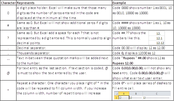
Do you remember the date & time formats we saw already? Excel provides few characters to represent each unit. For example: alphabet d represents date, m for month etc. In the same way, Excel has few representative characters to denote numbers. See the table below.

Note:

• If you enter more digits than placeholders, Excel displays all the digits.
• If you enter fewer digits than placeholders, Excel displays digits based on the characters above.
• If you enter more decimal digits than placeholders, Excel rounds off the decimals to number of placeholders.
• If you enter fewer decimal digits than placeholders, Excel displays digits based on the characters above.

What’s more? You can even display different colours for each section. See the available colours and codes below. You have to enclose colour codes in square brackets.

You can use one colour for each section. I have highlighted white colour cell with grey background (coz we cannot see white font in white background). Beautiful, isn't’ it?

Are these 8 standard colours not enough for you? Well, Excel has a solution for this too. Excel has colour codes along with colour names. If you use these codes, Excel’s 56 colours palette is at your disposal. Using [Black] as same as [color 1]

Comparison

You can create conditions using the basic comparison operators. Allowed operators are below.

Example: In a case when you have to display decimals if number entered in the cell is less than one, round off numbers to multiples of 1000 if it is more than 10000, you can use these conditions.

Conditions must be enclosed in brackets. Semi colon is used to separate different conditions. In the next post, we will see few examples on how to build format codes.

Custom Time Format

We saw how to build a custom date format in our earlier post. Now let’s see how to build custom time formats. Remember the coding table? I gave extract of time related codes here.

Let’s see how to code a custom time format.

Display as 11:15:10 AM

We need code for

• A 2 digit hour
• 2 digit minute
• 2 digit second
• AM or PM

So our code would be

hh:mm:ss AM/PM

Display Only Hours or Minutes or Seconds

You will just have either hh or mm or ss in the code as per your need.

But the problem in the above format is that you will see only hours equal to or less than 23, minutes equal to or less than 59 and seconds equal to or less than 59. Once the seconds cross 59, it will become 0 and minutes will be increased by 1. When minutes count crosses 59, it will become 0 and hours will be increased by 1. Similarly, when hours cross 23, it will become 0 and days count will be increased by 1.

If you just want to see the total hours (like 38 hours), total minutes (like 75 minutes) or total seconds (like 145 seconds) between two date/time values: we shall enclose the respective character in closed brackets. For example, if you want to see how many hours elapsed between two date / time values, below will be the code.

[hh]:mm:ss

A comparison between different formats is given below. In third row, I am trying to subtract second date from first date.

Note that in third column, since hours will not be added to days count even when it crosses 24 hours, you should not have code to show days count. If you input day’s representative code, [hh] will be considered as hh only i.e. hours more than 24 will be added to days count.

Accordingly, if you enclose minute’s code in brackets, you should not have hour’s code; if you enclose second’s code in brackets, you should not have hour’s and minute’s code.

In similar fashion, you can arrive at number of minutes or number of seconds elapsed by enclosing those codes in brackets.

Explore other combinations you require. If you are not able to make up the one you want, just let me know. Happy Learning!!

Custom Date Format

In our previous post, we saw couple of things about dates & times. There are formats available to display a number as a date / time. However, If you couldn't find the date or time format you are looking for in the built in list, you can create one of your own. Read on to know more about custom date and time formats.

To Create Custom Date And / Or Time Format

Press Ctrl+1 > Custom tab > Click one of the date format code available under Type or type your own code as explained in the next section.

In the Custom type, you can see some more date/time formats at your disposal (you have to scroll down to see them). See if one of them is what you want. If you find the one you wanted, click it and click OK. But if you want more, why wait, read on.

To get the desired format you want, you have to write the code that represents it in Type: box. Don’t worry; this code is not complex like VBA code. See below to know what this code is.

Understand the Format Code

Format code can be built using characters specified to represent each category of displayed values. For example: alphabet h denotes hours, s denotes seconds etc. Below is the list of all characters used for date and time.

• You can combine one or more code items to get the format you want.
• You can use characters like space, : (colon), / (forward slash), - (hyphen) to separate days, months, years etc.
• Notice that m is used both for months and minutes. If you place m right side of h, it is treated as minutes. Otherwise, it is to represent months.
• If you want a particular text to be displayed, you can enclose your text in double quotes (Ex: “Total is: ”)

Let’s build a couple of custom formats using above info.

Display as Monday, 24 March 2014 03:51 PM

Let’s divide what we need into parts. We need:

• A complete day in text i.e. Monday
• A comma
• A Space
• Date in 2 digit number i.e. 24
• A Space
• Complete Month in text i.e. March
• A Space
• Year in 4 digits i.e. 2014
• A Space
• Hours in 2 digits i.e. 03
• A colon
• Minutes in 2 digits i.e. 51
• A Space
• Time of the day (AM or PM)

Looking at the table above, you can get code characters you need for each one of above items. Let’s summarize them.

We use a space character to get space and colon character for a colon. So our final code will be

dddd, dd mmmm yyyy hh:mm AM/PM

Try it, copy above line in to the Type: field and click OK. Enter a date and see how it is displayed. Notice the formula bar too.

Display as The Date Is: 24 March 2014

Let’s see what we need to display above format.

• A text i.e. The Date Is:
• 2 digit date i.e. 24
• Full month i.e. March
• Four digit year i.e. 2014

From the table above, we can deduce the code as below.

"The Date Is" : dd mmmm yyyy

Copy above line in to the Type: field and click OK. Enter a date and see how it is displayed, notice the formula bar.

You can see the text you entered on the face of excel. But formula bar doesn't show it. You can use this cell in any formula just like a normal number.

There are number of date and time formats you can build based on your needs. Above is the required information to give you a head start. Try more combinations for yourself. Happy learning!!!

About Date Formatting

When you enter 2/2 in a cell, Excel thinks smart and will format the cell value as 2-Feb. As I mentioned in an earlier post, Excel treats any cell entry in only 2 categories i.e. a number and a non-number. Date is just a number that is in disguise as date. Let’s see in detail.

We will enter couple of dates in few cells like below. 

Once you are done entering the dates, notice the Number Format box. It will show Date as applied format for these cells. Select all these dates, and change the number format to General. (Click Home tab > Number group or press Ctrl+1). These dates will now be changed as in below picture.

24^th Mar 2014 became number 41722 and so on. What is this?

1 January 1900

Excel uses 1900 date system by default. That means, it thinks the world has started on 1^st Jan 1900. This date is considered as 1 and each day after this is increased by 1. So 1 Jan 1900-12:00:00 AM is 1, 2^nd Jan 1900-12:00:00 AM is 2….and so on. In that order 41722 comes to 24^th Mar 2014.

Excel also has another date system called 1904. We will see about that sometime later but not here.

Alright, so one day is represented by 1. Did you get the doubt, what about hours, minutes & seconds, how to show them? Simple! To show fractions of a day, 1 is to be divided by respective fraction. For example, if you want an hour, divide 1 by 24, result denotes an hour. You can do math for other fractions. See below for the fractions, rounded off to 6 decimal points.

To facilitates calculations, 0 (zero) is treated as 0 Jan 1900-12:00:00 AM, though date 0 Jan is not logical. So when you add dates or subtract dates, what’s happening really is addition or subtraction of 2 numbers behind the scenes. Now you know how you can add/subtract dates from each other. 

Now let’s see how few numbers will be displayed as dates.

I used a custom format “dddd, d mmmm yyyy hh:mm:ss AM/PM” to show above example. (I will write about this format shortly).

There are various built-in date and time formats available in Excel. Check out different formats by following the below sequence.

To Set Date Format

Press Ctrl+1 > Date tab > Select appropriate option under Type

There are around 13 different types available for Date format. Choose the one you fancy and your date in that cell will show just like it.

To Set Time Format

Press Ctrl+1 > Time tab > Select appropriate option under Type

There are 3 types available for Time formatting.

Human needs are unlimited, right? If you are not satisfied with built-in formats, Excel also facilitates you to create your own. We will see about that in next post.

Cell Formatting Options

Excel is smart (well, sometimes). It automatically applies formats as you type anything in a cell. You type 1/2 in a cell; Excel turns it as 1-Feb (date format). You enter 1 1/2 (notice the space in between); Excel shows it as fraction format. Any input that Excel doesn’t recognise as a number will be taken as text. We fairly know about various formats available in Excel. Let’s see a quick overview of them.

There are more than 10 types of built-in formats available in Excel. But digest this; Excel categorizes any value you enter in a cell in just 2 type’s viz. a number and a non-number. A number can be further formatted to “display” the way we want on the face of Excel but the underlying number will not change. To understand what I mean, see the below picture.

I entered 10 in all the cells and formatted them using different formats as mentioned in third column. Same number is shown in different formats. We can notice the formula bar selecting each cell, no matter what is shown in the cell, formula bar always contains 10 (except for date, time & percentage).

So it is clear that any format you apply over a cell, ONLY appearance of that cell value will be changed accordingly but not the actual value.

General

General format is default format of Excel. For the most part, numbers that are formatted with the General format are displayed just the way that you type them. However, if the cell is not wide enough to show the entire number, the General format rounds off numbers that have decimals. The General number format also uses scientific (exponential) notation for large numbers (12 or more digits)

Select the cell(s) > Press Ctrl+1 > Number tab > under Category, select General to apply this format.

Number

Number format will place 2 decimal points by default to the value you enter. You will have options to increase / decrease the decimal points, to place a thousand separator and to select a way how negative numbers appear.

Select the cell(s) > Press Ctrl+1 > Number tab > under Category, select Number to apply this format.

Explore other formats and options based on your convenience. We will see more about few formats that are worth discussing in one of our future posts. See you!!