VBA - Application.InputBox

We saw about InputBox function in our previous post. We learnt that you cannot restrict user to enter a particular type of values in InputBox. Of course, you can write couple of lines of code to validate user entry, but wouldn’t it be nice if your InputBox itself does that validation for you?

Application.InputBox method is at your rescue. Let’s see what it is and how to use it.

Application.InputBox calls a method of the Application object. A plain entry of InputBox in the code calls a function of InputBox that we discussed in our previous post.

Application.InputBox is a powerful tool to restrict the users to enter particular type of values. It also gives more flexibility to choose from various types of values that normal InputBox cannot. For example: you can let user select a range using Application.Input which is simply not possible with standard InputBox.

Also, returned value form the Application.InputBox method is a variant as opposed to a text string that is returned by plain InputBox. A variant can represent any kind of variable data type we discussed in post on varaibles. For example: it can hold a text string, a formula, a Boolean value, a complete Range reference and an array etc.

Syntax

Application.InputBox(Prompt, Title, Default, Left, Top, HelpFile, HelpContextID, Type)

Application.InputBox: This is the key word to call this method.

Prompt: Mandatory. Whatever you enter in this argument will be displayed to the user. If you are entering a string in prompt, you will have to enclose that string with double quotes. You can also pass one of the variable values as an argument for this.

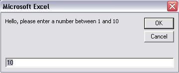
Title: Optional. This is the text shown on top of the message box. If omitted, “Input” will be shown. Notice the difference. In InputBox, if this argument is omitted “Microsoft Excel” is shown.

Default: Optional. This is shown as default value in the InputBox.

Left: Optional. Specifies an x position for the dialog box in relation to the upper-left corner of the screen

Tops: Optional. Specifies a y position for the dialog box in relation to the upper-left corner of the screen

Helpfile: Optional. If you notice the alert produced by Excel will have either a help button or a question mark button on the alert. Those are to display a help file that is saved with the program. If you have a help file created for your message box, you can provide that here. But creating a help file deserves multiple separate posts but that’s not our concerns at this point of time. You can conveniently ignore this.

HelpContextID: Optional. It is the number of the topic to be displayed from helpfile. If this is provided, helpfile is mandatory (quite obvious)

Type: This is where it is way more powerful than plain InputBox function. Type specifies the return data type. If this argument is omitted or number 2 is entered, the dialog box returns text (which replicates plain InputBox function). You have below options to pass on for this argument.

Notes:

• It is mandatory to assign the Application.InputBox function to a variable if you are using more than one argument
• If you want to omit any argument and move to next one, you should include a comma
• You can allow different types of data input by combining the values with plus sign. For example: if you want to allow numbers and text too in a box, your Type argument would be 1+2.

Let’s see this in action by few examples.

Example 1: Display a message to the user asking to enter a number between 1 and 10.

Sub Test()
Application.InputBox("Enter a number between 1 and 10")
End Sub

Running the code displays below box. This is just like InputBox in operation. You are not restricting any user entry.

Notice the prompt “Input” and placement of buttons at the bottom. This is different if you compare with InputBox dialogue (below picture is copied from InputBox post)

Example 2: Display a message to the user asking to enter a number between 1 and 10. With number 10 entered already in the box that will be displayed.

Sub Test()
MyInput = Application.InputBox("Enter a number between 1 and 10", , 10)
End Sub

Notice the code: Since I am using more than one argument, I assigned Application.InputBox to MyInput variable. As third argument, I entered number 10 which is what I wanted in the box.

Executing code above will display below box.

Number 10 pre-entered in the box will help user if that is what commonly used. It reduces few key presses from the user. If user wants to enter a different number, he can delete existing and enter whatever he wants.

Example 3: Let user select a range of cells.

Sub Test()
MyInput = Application.InputBox("Select a range", , , , , , 8)
End Sub

Running the above code would show up a box and you can click on any cell or cells in Excel, address of that cells is reflected in dialogue box like a formula as shown below.

Example 4: With the above settings, restrict user to enter only numbers.

Sub Test()
MyInput = Application.InputBox("Enter a number between 1 and 10", , 10, , , , , 1)
End Sub

Notice the commas; I am skipping the arguments by placing a comma for each argument. For last argument, I entered number 1 which represents the number Type. After executing this code, a dialogue box just like above will be displayed. However, if the user enters anything other than a number, it will show an error. This process continues until user clicks Cancel or enters a number.

Below is the error displayed if I enter some text in this box and click OK.

Values returned by Application.InputBox can be used just like how we used InputBox returned values. For example, you can let user select few cells and apply formatting to those cells only or ask user to enter a number (let’s call it n) and highlight every n^th row in the sheet etc.

We can see Application.InputBox in action while we move ahead in our learning and start writing complex codes to achieve big tasks. Till then, happy learning!!

VBA - Input Box

Thank you readers for encouraging my posts on Excel. With this post, this blog now has 100 posts and many more to go. Let's spread the knowledge. Cheers!!!!

We saw about MsgBox in one of our previous posts. MsgBox is used to alert user with some information. We can also provide some buttons such as Yes, No, Retry etc for the user to click. According to user response, we can continue with next steps of macro.

In some cases, it might not be enough to just get user click a button. You may have to solicit some information from the user for further action. For example: you may have to get a name from the user and use that name in a subsequent procedure. MsgBox function falls short here as it can only offer buttons to click.

In such cases, InputBox function is your friend. This function is similar to MsgBox with an additional functionality to solicit input from user. InputBox function displays a prompt in a dialog box, waits for the user to input text or click a button, and returns a string containing the contents of the text box.

InputBox syntax

InputBox(prompt[, title] [, default] [, xpos] [, ypos] [, helpfile, context])

InputBox: This is the key word to call Input Box

Prompt: Mandatory. Whatever you enter in this argument will be displayed to the user. If you are entering a string in prompt, you will have to enclose that string with double quotes. You can also pass one of the variable values as an argument for this. Do you remember the line we used in variables post?

Title: Optional. This is the text shown on top of the input box. If omitted, “Microsoft Excel” will be shown.

Default: Optional. This is shown as default value in the InputBox.

Xpos: Optional. This is a number that specifies the horizontal distance of the left edge of the dialog box from the left edge of the screen. If xpos is omitted, the dialog box is horizontally centred.

Ypos: Optional. This is a number that specifies, the vertical distance of the upper edge of the dialog box from the top of the screen. If ypos is omitted, the dialog box is vertically positioned approximately one-third of the way down the screen.

Helpfile: Optional. If you notice, the alert produced by Excel will have either a help button or a question mark button on the alert. Those are to display a help file that is saved with the program. If you have a help file created for your box, you can provide that here. But creating a help file deserves multiple separate posts but that’s not our concerns at this point of time. You can conveniently ignore this.

Context: Optional. It is the number of the topic to be displayed from helpfile. If this is provided, helpfile is mandatory (quite obvious)

Notes:

• It is mandatory to assign the InputBox function to a variable if you are using more than one argument.
• If you want to omit any argument and move to next one, you should include a comma.

Let’s see the InputBox in action with few examples.

Example 1: Display a message to the user asking to enter a number between 1 and 10.

Sub Test()
InputBox ("Hello, please enter a number between 1 and 10")
End Sub

Executing the code above will display a dialogue like below.

In the bottom of the above box, user can enter anything and / or click OK or Cancel buttons. We will see how to work with user response shortly.

Example 2: Display a message to the user asking to enter a number between 1 and 10. With number 10 entered already in the box that will be displayed.

Sub Test()
Dim MyInput As String
MyInput = InputBox("Hello, please enter a number between 1 and 10", , 10)
End Sub

Notice the code: Since I am using more than one argument, I am declaring a variable MyInput and assigned InputBox to that variable. And I used a comma to skip second argument. As third argument, I entered number 10 which is what I wanted in the box by default.

Executing code above will display below box.

Number 10 pre-entered in the box will help user if that is what commonly used. It reduces few key presses from the user. If user wants to enter a different number, he can delete existing and enter whatever he wants.

When the user clicks OK button, whatever is entered in the box will be assigned to the variable. If Cancel button is clicked then our variable get a null string (empty or nothing is represented by “” i.e. two double quotes with nothing in-between)

Problem with InputBox is that you cannot define the buttons you need. OK and Cancel buttons are always displayed.

Work With User Response

InputBox returns user entry as a text string. Using this string; you can further write code that uses it. Let’s extend our example code above to show the user entered value back to him in an MsgBox for confirmation.

Sub Test()
Dim MyInput As String
MyInput = InputBox("Hello, please enter a number between 1 and 10", , 10)
If MyInput = "" Then 'User didn't enter anything or clicked cancel
    MsgBox ("You entered nothing")
Else 'Ok. something is entered
    MsgBox ("You entered" & MyInput & vbCrLf & "Click OK to Proceed")
End If
End Sub

Running above code displays an input box first (refer to above picture). Based on user action, there will be subsequent message boxes.

If user clicked Cancel button or didn’t not enter anything and clicked on OK button, below message is displayed.

If user entered something (not necessarily a number between 1 and 10) and clicked on OK button, below message is displayed. (Of course, with whatever user entered in place of 10)

As mentioned above, InputBox returns anything entered in it as a string i.e. as text. Even if you enter a number 10 as above, you cannot use it in subsequent calculations as a number. If you are sure that only number is entered, multiply the string with 1 in your code. That would force the number in string to be identified as a number.

Sub Test()
MyInput = InputBox("Hello, please enter a number between 1 and 10", , 10) * 1
End Sub

But remember, above code will result into an error if what is entered in the InputBox is not a number.

MsgBox & InputBox are the two basic dialogues used to solicit user’s response. Both have their own limitations, for example in InputBox, you cannot restrict the user to enter only a number. You cannot customize appearance of these boxes etc.

But there are alternatives. If you are looking to restrict what user enters, you can use Application.InputBox (note that what we saw above is a plain InputBox. With Application qualifier, a different function is called altogether). We will see about this in our next post.

You can make your own designed message boxes and input boxes using UserForms. We will see about them eventually. Till then, explore what we discussed on this series till now. Cheerio!!!

Minimise The Ribbon

This article is applicable only to Excel 2007 and later versions where Microsoft Office fluent Interface (aka Ribbon) is implemented. Ribbon replaced the earlier menus and it is quite handy.

There is no way to delete or replace the Ribbon with the toolbars and menus to appear like earlier versions of Microsoft Office. However, you can minimize the Ribbon to make more space available on your screen. When you minimise ribbon, tabs are visible but not the options under those tabs.

Ribbon When Visible

Ribbon When Minimised

Minimising ribbon shows few rows more in the sheet than when it is visible. However, you can still use all the key board shortcuts to do your job. You can also click any tab once when the Ribbon is minimised to get the ribbon temporarily visible.

How to Minimise Ribbon

Easiest Way

Just press Ctrl and F1 together. The Ribbon is gone until you press the same combination again.

Easy Way

With the mouse pointer, double click the active tab name. For example, if Home tab is activated, double click on the word Home. Double click on any active tab again to get the Ribbon back.

Long Way

Click on Quick Access Toolbar (QAT) drop down button.

In the drop down, click on More Commands… In the dialogue box that opens up, select All Commands in Choose commands from dropdown. Locate Minimize the Ribbon in box that is below the dropdown and click Add >>. Click OK.

Now you should be able to see a new button added to your QAT.

Click on the button to minimise the ribbon or make it visible.

VBA Way

Copy the code below to a code window and execute. That should minimise the ribbon. Run again to make it normal.

Sub HideRibbon()
    CommandBars.ExecuteMso "MinimizeRibbon"
End Sub

VBA Way 2

Copy below code and paste in a code window. Go to Excel and run macro from View > Macros (i.e. not from the code window directly)

Sub HideRibbon()
    Application.SendKeys ("^{F1}")
End Sub

Change the Default View of Newly Created Sheet

When you add a new sheet, Excel by default shows the newly created sheet in Normal mode (as opposed to Page Layout view or Page Break view). If you want to change this behaviour and let Excel opens in the mode you want, change the default setting as below.

Excel 2010 and later:

File tab > Options > General > When creating new workbooks segment > select mode you like in the Default view for new sheets drop down. Options available are Normal View (default), Page Break Preview, and Page Layout View.

Excel 2007:

Click the Microsoft Office button > Excel Options > Popular tab > When creating new workbooks segment > select mode you like in the Default view for new sheets drop down. Options available are Normal View (default), Page Break Preview, and Page Layout View.

This feature was introduced in Excel 2007. Users of earlier versions are out of luck here.

Use A Template For Pre-Applied Formatting

If you need to use a specific format for all your files, you can try saving the format you want as a template file. and whenever a new Excel file is created, you can directly apply template rather than making changes manually. For example: if you always want gridlines to be off when you create a new workbook or want to have a standard text for header etc, you can use templates.

One of my friends in billing team spends most of his time preparing invoices in Excel and printing them. He keeps an invoice format in a file on his desktop and opens that each time. He could save some time if he can save that invoice format as a template and keep it in start-up folder so that every time he opens up an Excel file, it opens with his invoice format by default. Let’s see how to do that.

1. Create a new workbook
2. Apply all the formatting you need (cell format, styles, sheet format), data validation settings etc to this workbook
3. Press Ctrl+S
4. In the Save in field, locate XLSTART folder. This folder can be found in one of the following locations depending on your operating system.
• Windows XP: C:\Documents and Settings\<username>\Application Data\Microsoft\Excel\XLStart
• Windows Vista: C:\Users\<username>\AppData\Local\Microsoft\Excel\XLStart
• Windows 7: C:\Program Files\Microsoft Office\Office\XLStart
5.  In the File name field, type Book
6. In the Save As window, Select Excel Template (In Excel 2007 onwards) / Template (In Excel 2003 and below) in Save as type field drop down list.
7. Click OK.

That’s it. From now on, whenever you create a new workbook, it will contain all the formatting you applied in step 2 above.

The ClearType Font

Caution: Techie terms ahead

What is ClearType

ClearType is a technology of showing text in a font. ClearType is owned by Microsoft and was introduced first in 2000.

How it Works

Normally, the software in a computer treats the computer’s display screen as a rectangular array of square, indivisible pixels, each of which has an intensity and color that are determined by the blending of three primary colors: red, green, and blue. However, actual display hardware usually implements each pixel as a group of three adjacent, independent subpixels, each of which displays a different primary color. Thus, on a real computer display, each pixel is actually composed of separate red, green, and blue subpixels. 

If the computer controlling the display knows the exact position and color of all the subpixels on the screen, it can take advantage of this to improve the apparent resolution in certain situations. If each pixel on the display actually contains three rectangular subpixels of red, green, and blue, in that fixed order, then things on the screen that are smaller than one full pixel in size can be rendered by lighting only one or two of the subpixels. For example, if a diagonal line with a width smaller than a full pixel must be rendered, then this can be done by lighting only the subpixels that the line actually touches. If the line passes through the leftmost portion of the pixel, only the red subpixel is lit; if it passes through the rightmost portion of the pixel, only the blue subpixel is lit. This effectively triples the horizontal resolution of the image at normal viewing distances; the drawback is that the line thus drawn will show color fringes (at some points it might look green, at other points it might look red or blue).

ClearType uses this method to improve the smoothness of text. When the elements of a type character are smaller than a full pixel, ClearType lights only the appropriate subpixels of each full pixel in order to more closely follow the outlines of that character. Text rendered with ClearType looks “smoother” than text rendered without it, provided that the pixel layout of the display screen exactly matches what ClearType expects.

Why Are We Bothered 

Microsoft had implemented ClearType font in all MS Office products from 2007 and onwards. This is on by default. If at all you feel your font is rendered bit blurry, you may want to try switching off this feature.

According to a study at the University of Texas, ClearType "may not be universally beneficial". The study notes that maximum benefit may be seen when the information worker is spending large proportions of their time reading text (which is not necessarily the case for the majority of computer users today). Additionally, over one third of the study participants experienced some disadvantage when using ClearType. Whether ClearType, or other rendering, should be used is very subjective and it must be the choice of the individual, with the report recommending "to allow users to disable [ClearType] if they find it produces effects other than improved performance".

How to Disable / Enable ClearType 

Excel 2007:

Click the Microsoft Office button > Excel Options > Popular tab > Top options for working with Excel segment > clear the Always Use ClearType check box.

Excel 2010 and later:

File tab > Options > General > User Interface options segment > clear the Always Use ClearType check box.

Follow the same steps but check the box if you want to enable this feature.

Points to Remember

You will have to close all the Office applications that are open while changing this feature to take effect. 

Microsoft do not recommend to turn off this feature. As a workaround, you can use Microsoft’s ClearType tuning tool. More information can be found here.

Change the Default Font & Size

By default, Excel uses Calibri font with 11 pt size (10 pt if you use Excel 2003) for any new workbook you create. Of course, you can change the formatting for each book / sheet whenever you like. But your company uses a particular font in all the reports (other than Calibri) and you want that font as your default font? Read on.

This post is useful if you want to change the default font and size so that each time you create a new workbook, your chosen font is the default.

Excel 2010 and later:

File tab > Options > General > When creating new workbooks segment > select font you like in the Use this font drop down. Select size of the font you want as default in the Font size drop down list.

Excel 2007:

Click the Microsoft Office button > Excel Options > Popular tab > When creating new workbooks segment > select font you like in the Use this font drop down. Select size of the font you want as default in the Font size drop down list.

Excel 2003:

Tools menu > Options > General tab > select a font in the Standard font drop down box. In the Size box, type or click a font size.

Points to remember:

1. You must restart Microsoft Office Excel to begin using the new default font and font size.
2. The new default font and font size are used only in new workbooks that you create after you restart Excel. Existing workbooks are not affected.

Change Default User Name

Excel by default picks up the system login ID as the user name. All the Excel files you create will be stamped with your login name as author. Also, when you insert a comment, every comment by default starts with the user name.

If you don't like the default logic ID to be your Excel user name, you can change it and put any name you fancy. Let's see how to do it.

Excel 2010 and later:

File tab > Options > General > Personalize your copy of Microsoft Office segment > type a name in the User Name.

Excel 2007:

Click the Microsoft Office button > Excel Options > Popular tab > Personalize your copy of Microsoft Office segment > type a name in the User Name.

Excel 2003:

Tools menu > Options > General tab > > type a name in the User Name.

Points to remember:

1. User Name cannot be more than 52 characters. You can have special characters too in the name.
2.  If you keep user name field blank, Excel automatically places the Windows user name.
3. Changing the user name will effect the future workbooks. Files already saved with earlier user name will not be updated.

VBA - Error Trapping

When an error occurs while executing the code, VBA treats that error as fatal and stops executing the code then and there, with an error alert message to the user. While at times this is what you may want, most of the times you will just have to continue running the code and do other jobs that macro was supposed to do. For this, we have to use what is called an Error Trapping. VBA provides ways to tackle with that error without interrupting the code. Let’s see what options we have to do that.

On Error Statement

This statement enables error-handling routine and you can specify from where the code should continue executing. We have 3 options to provide such location.

On Error Resume Next

This tells VBA to ignore the error and continue running the code from immediate next line of code following the line where the error occurred.

This error handler will be active through out your code. No matter how many times errors occurr in your procedure, VBA always executes the next line. But be careful, with this line, VBA ignores any kind of error. If you don’t take care, it may result into ignoring few errors that should not be ignored.

On Error GoTo line

This enables the error-handling routine to start at the line specified in the argument. The line argument is any line label or line number. The specified line must be in the same procedure as the On Error statement; otherwise, a compile-time error occurs.

Note that, on first occurrence of first error, VBA starts executing the code from line given as argument and continues executing the lines below it till the End Sub.

Once executed, error handler will be disabled for further use. That means, On Error GoTo statment can be used for only one error in a procedure.

On Error GoTo 0

Disables any error handler that is in the current procedure!

Let's see the error handling through an example. We will deliberately do something that causes an error. How about try to enter some value in a protected sheet and that will cause an error? Copy/Paste the below code to your module! Protect the active sheet. Click anywhere on the code in VBA and press F8 repeatedly to run the macro line by line. On each press of F8, you can notice where the focus is going.

Example –On Error Resume Next

Sub Test()
On Error Resume Next 'Defining the error trapping, on error focus should go to next line
ActiveCell.Value = 1000 'try to enter some random value in active cell
If Err.Number <> 0 Then 'check if error occurred?
    MsgBox ("Error Occurred") 'Yes? then message box saying so
Else
    MsgBox ("Done") 'No? Then all done.
End If
End Sub

Run this code by repeatedly pressing F8. Now you see that no matter what, focus will always go to the next line. We are trapping the error by If-Then-Else-End If statements.

Example –On Error Goto line

Sub Test()
On Error GoTo ErrorHandler 'Defining the error trapping, focus should go to a line named ErrorHandler below
ActiveCell.Value = 1000 'try to enter some random value in active cell
Exit Sub 'If no error, procedure should stop here

ErrorHandler: MsgBox ("Sorry, Error " & Err.Number & " Occurred") 'This line contains what to do in case of error
End Sub

If you noticed, from ActiveCell.Value = 1000 line, focus will change to ErrorHandler, as there will be an error when executing that line and we asked VBA to go to ErrorHandler on error occurrence. On one more press F8, a message box is shown informing the error number to the user.

Err Object

Wherever there is an error, VBA keeps that error information in Err object. You can use this information to know more about the type of error. You can in turn display the information to the user as we did in our earlier code. Err.Number provides the system assigned number of this error. There is also Err.Description will provide the description of the error. See other options available under Err object and explore.

VBA - If Then Else Endif

Do you remember the Excel built-in function IF? You can provide a condition to be evaluated by IF and provide a calculation / value if result is TRUE and provide a different calculation / value if result is FALSE. In similar lines, VBA also provides a feature i.e.. IF statement. Syntax for this is as below.

Form 1 – In One Line – Without Else Condition

If condition Then statement

If: is the key word to call this feature

Condition: what do you want to evaluate. You can give one or more conditions to evaluate (we will see how)

Statement: what if condition is met.

We are not defining what to do if condition is not met so macro will do nothing (moves to next available line of code).

Example: If ActiveCell.Value = 5 Then MsgBox(ActiveCell.Value)

This form is best used if you just want to evaluate one condition followed by single line action if condition is true. No action if condition is false.

Form 2 – In One Line - With Else Condition

If condition Then statement [Else elsestatement]

Other key words are similar as above form.

Elsestatement: What if condition is not met

Example: If ActiveCell.Value = 5 Then MsgBox(ActiveCell.Value) Else MsgBox(“No Match”)

This form is best used if you just want to evaluate one condition followed by single action if condition is true and a single line action if condition is false.

Form 3 – Multiple Lines - Without Else Condition

If condition Then

statement

Endif

Example:

If ActiveCell.Value = 5 Then
    MsgBox(ActiveCell.Value)
End If

Form 4 – Multiple Lines – With Else Condition

If condition Then

statement

Else

elsestatement

End If

Example:

If ActiveCell.Value = 5 Then
     MsgBox(ActiveCell.Value)
Else
     MsgBox(“No Match”)
End If

Form 5 – Multiple Lines - Multiple Else conditions

If condition Then
     statement
Elseif condition Then
     Elsestatement
Elseif condition Then
     Elsestatement
……………………….
Else
statement
End If

Example:

If ActiveCell.Value = 5 Then
      MsgBox(ActiveCell.Value)
Elseif ActiveCell.Value = 4 Then
      MsgBox(Application.UserName)
Elseif ActiveCell.Value = 3 Then
      MsgBox(“Welcome To The World”)
Else
      MsgBox(“Bye Guys”)
End If

Above examples are pretty much self explanatory. Copy them to a VBA module, enter a value in a cell and execute the macro. We will use many If Then Else statements in our forth coming macros. Stay tuned!!

Control The Cursor Movement on Pressing Enter

Typically, whenever you press Enter in Excel, cursor will move one box down (there are few exceptions, that’s not the point for this post). Few know that you can command Excel to behave differently upon pressing Enter viz. do nothing, go Up, Left or Right. Let’s see how to do that.

Excel 2010 and later:

No Cursor Movement after Enter

File tab > Options > Advanced tab > Editing options segment > clear the check box After pressing Enter, move selection > OK.

To Move Cursor In a Direction

File tab > Options > Advanced tab > Editing options segment > check the check box After pressing Enter, move selection > and select the direction you want the cursor to move in Direction drop down. Available options are Down, Right, Up and Left > OK.

Excel 2007:

No Cursor Movement after Enter

Click the Microsoft Office button > Excel Options > Advanced tab > Editing options segment > clear the check box After pressing Enter, move selection > OK.

To Move Cursor In a Direction

Click the Microsoft Office button > Excel Options > Advanced tab > Editing options segment > check the check box After pressing Enter, move selection > and select the direction you want the cursor to move in Direction drop down. Available options are Down, Right, Up and Left > OK.

Excel 2003:

No Cursor Movement after Enter

Tools menu > Options > Edit tab > clear the check box Move selection after Enter > OK.

To Move Cursor In a Direction

Tools menu > Options > Edit tab check the check box Move selection after Enter > and select the direction you want the cursor to move in Direction drop down. Available options are Down, Right, Up and Left > OK.

Once you are done with above steps, press Enter in excel and see how the cursor is moving.

Live Preview

Excel 2007 introduced a concept called Live Preview. Using this, you can view how the format change you are about to make actually look like, even before applying that change. This saves you the time you would otherwise spend on applying various formats and removing the applied format if you don’t like it.

You can access this feature by hovering the mouse over desired format options and wait a second, Excel will automatically update the selection to show how that will look like once the highlighted format applied. You just need to click on those options if you fancy or move away from it if you don’t like. That’s all.

Example:

To check different font sizes: Select the cells you want to change font size and Home tab > Font group > click the Font Size box down-arrow, and then move the pointer over different font sizes. Observe the cells you selected, they will change the size as you hover the mouse.

You can preview font formatting, quick styles, picture formatting using this feature. If you are using Excel 2010, you can also preview the Paste commands such as Keep Source Column Widths, No Borders, or Keep Source Formatting.

Though this option is awesome, if you feel that you don’t require live preview, there is an option to turn this feature off. Let’s see how.

Excel 2007:

Click the Microsoft Office button > Excel Options > Popular tab > Top options for working with Excel segment > clear the Enable Live Preview check box.

Excel 2010 and later:

File tab > Options > General > User Interface options segment > clear the Enable Live Preview check box.

Follow the same steps but check the box if you want to enable this feature.

Use Custom Number Formats Across Workbooks

We have been seeing about how to create custom data/time & number formats in a series of posts.  If you follow those codes carefully, by now you must be able to create formats as you require. There is a problem with these custom formats. They will be saved in the workbook you created them in and will not be available for other workbooks. If you spent an hour to create a custom number and want to use it across all Excel books anytime, you will have to save that workbook you have the customer format as a template.

Templates can contain the sheets, default text (such as page headers and column and row labels), formulas, macros, styles, and other formatting you want in all new workbooks you create.

Once you create a workbook with your custom format, save it as a template as below.

• Click on File tab > Save As (Excel 2010) / Microsoft Office Button > Save As (Excel 2007) / File menu > Save As (Excel 2003)
• Save as type box, click Excel Template or Excel 97-2003 Template (Excel 2007 or later) / Template (Excel 2003 or lower)
• Give any name you want to this workbook and click Save.

Next time onwards, whenever you want your custom formatting required in a new workbook, you will have to create a new workbook using File tab > New > New from existing (Excel 2010) / Microsoft Office Button > New > New from existing (Excel 2007) / File menu > New > From existing workbook(Excel 2003).

If you think this is too much to do or want your custom format available whenever you open Excel, you may want to save your template in XLStartup folder or alternate startup folder.

Custom Number Format - Examples

We have been seeing about different formatting available in Excel. In the last post, we saw about the codes used for custom number formats. Let’s see few examples now on how to use the code we learnt.

Display Whole Positive numbers ONLY

Yeah, weird, but I want it. I want to display the contents of the cells only if they are positive whole numbers like 1, 2, 3...and so on. Any others like negative numbers, text or decimals should not be shown in the cell. Let’s see how to code them.

I will break down our logic in parts.

• We want positive numbers to display but no decimals
• We don’t want to show negative numbers
• We don’t want to show zeros
• No text either

From what we learnt from the code in last post,

• Every cell can have 4 parts of display.
• If we don’t want a part to display, we can just enter a semi colon in that place.
• To display numbers we can use any one of 0, # and ? depending on your need. I will use 0.

Following the above logic, I can deduce the below code.

0;;;

Select a cell and apply above custom format. Enter different types of data in the cell and see how Excel will display or hide them.

Similarly you can code to show only negative numbers (use ;-0;;) note the minus sign before zero;, display zeros only (use ;;0;) and to display text only (;;;@). Needless to say, you can use combination of two or more criteria, such as show only positive and negative numbers and hide zeros & text (use 0;-0;;).

To display numbers with up to 2 decimals, you will replace 0 in above codes with 0.00 and so on based on your requirement.

Show Positive Numbers in Green, Negative in Red, Zeros in Blue and Text in Yellow

[Green]0;[Red]-0;[Blue]0;[Yellow]@

Display Nothing

;;;

Always Display X Number of Digits (Leading Zeros)

Bank account numbers for example will have fixed number of digits. Account numbers that doesn’t have those many digits will be prefixed with leading zeros. Like, if fixed length is 10 digits and you enter 12345, Excel can show it as 0000123545. If that is your need, you can use below code.

0000000000;;;

Above code should contain those many zeros as the number of digits you want. It is coded not to show negative, zeros & text.

Below is the picture showing how positive, negative, zeros & text appearing under different format codes as given above.

Display Telephone Number Style 1-800-333-3333

0-000-000-0000

Entering 1800333333 in this cell will show the number as 1-800-333-3333.

Display Numbers in Thousands / Millions

Round Off To Nearest Millions / Thousands / Numbers Based On the Number Entered

[>=1000000]0,, ;[>=1000]0, ;0

Above code displays values greater than or equal to 1 million rounded to nearest one million. If the entered number is not greater than or equal to 1 million, but is greater than or equal to 1000, then the value is rounded to nearest thousand. If neither condition is met then the figure will be displayed rounded to the nearest whole number.

Try different combinations in the code and explore it for yourself. Remember, you will learn excel better by doing trial and error yourself. But if you tried and couldn't get some format you needed, let me know. Happy Learning!!

Custom Number Format - Introduction

Note that formatting a number will ONLY change the appearance of it. That is, how you see the number on the screen changes but actual number you enter is NOT changed. We already saw how to build custom date & time format. So we are familiar with codes that represent the data.

A number format is coded in 4 parts. Each part of the code represents display format for positive numbers, negative numbers, zero values, and text respectively. Each of the part is separated by a semicolon (;). Syntax of this format is as below.

<POSITIVE>;<NEGATIVE>;<ZERO>;<TEXT>

You needn't write code for all 4 parts of the number. Excel has defaults and it can manage without coding few parts specifically. Let’s see what rules apply here.

• If you enter one code section – Excel take it for all the numbers (same format for positive, negative & zeros), default formatting for text
• If you enter two sections – First part is considered for positive numbers & zeros, second part is for negative numbers. Default formatting for text
• If you enter three sections – First part is considered for positive numbers, second part is for negative numbers, third for zeros. Default formatting for text
• If you want to skip a particular section, you place a semicolon for that section.

Do you remember the date & time formats we saw already? Excel provides few characters to represent each unit. For example: alphabet d represents date, m for month etc. In the same way, Excel has few representative characters to denote numbers. See the table below.

Note:

• If you enter more digits than placeholders, Excel displays all the digits.
• If you enter fewer digits than placeholders, Excel displays digits based on the characters above.
• If you enter more decimal digits than placeholders, Excel rounds off the decimals to number of placeholders.
• If you enter fewer decimal digits than placeholders, Excel displays digits based on the characters above.

What’s more? You can even display different colours for each section. See the available colours and codes below. You have to enclose colour codes in square brackets.

You can use one colour for each section. I have highlighted white colour cell with grey background (coz we cannot see white font in white background). Beautiful, isn't’ it?

Are these 8 standard colours not enough for you? Well, Excel has a solution for this too. Excel has colour codes along with colour names. If you use these codes, Excel’s 56 colours palette is at your disposal. Using [Black] as same as [color 1]

Comparison

You can create conditions using the basic comparison operators. Allowed operators are below.

Example: In a case when you have to display decimals if number entered in the cell is less than one, round off numbers to multiples of 1000 if it is more than 10000, you can use these conditions.

Conditions must be enclosed in brackets. Semi colon is used to separate different conditions. In the next post, we will see few examples on how to build format codes.