Note that formatting
a number will ONLY change the appearance of it. That is, how you see the number
on the screen changes but actual number you enter is NOT changed. We already
saw how to build custom date & time format. So we are familiar with codes that
represent the data.
A number format is
coded in 4 parts. Each part of the code represents display format for positive
numbers, negative numbers, zero values, and text respectively. Each of the part
is separated by a semicolon (;). Syntax of this format is as below.
<POSITIVE>;<NEGATIVE>;<ZERO>;<TEXT>
You needn't write
code for all 4 parts of the number. Excel has defaults and it can manage
without coding few parts specifically. Let’s see what rules apply here.
- If you enter one code section – Excel take it for all the numbers (same format for positive, negative & zeros), default formatting for text
- If you enter two sections – First part is considered for positive numbers & zeros, second part is for negative numbers. Default formatting for text
- If you enter three sections – First part is considered for positive numbers, second part is for negative numbers, third for zeros. Default formatting for text
- If you want to skip a particular section, you place a semicolon for that section.
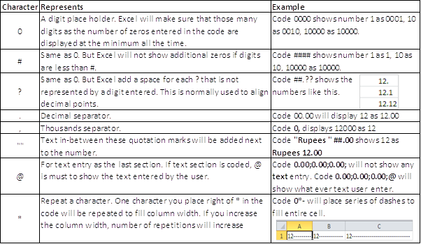
Note:
- If you enter more digits than placeholders, Excel displays all the digits.
- If you enter fewer digits than placeholders, Excel displays digits based on the characters above.
- If you enter more decimal digits than placeholders, Excel rounds off the decimals to number of placeholders.
- If you enter fewer decimal digits than placeholders, Excel displays digits based on the characters above.

You can use one colour for each
section. I have highlighted white colour cell with grey background (coz we
cannot see white font in white background). Beautiful, isn't’ it?
Are these 8 standard colours not
enough for you? Well, Excel has a solution for this too. Excel has colour codes
along with colour names. If you use these codes, Excel’s 56 colours
palette is at your disposal. Using [Black] as same as [color 1]
Comparison
You can create conditions using the
basic comparison operators. Allowed operators are below.

Example: In a case when you have to
display decimals if number entered in the cell is less than one, round off
numbers to multiples of 1000 if it is more than 10000, you can use these
conditions.
Conditions must be enclosed in
brackets. Semi colon is used to separate different conditions. In the next post, we will see few
examples on how to build format codes.
No comments:
Post a Comment