Functions: Working with Arrays

Hi there. This is last post for this year. Let's say bye bye to year 2013 and welcome 2014 with heart full of joy.

As we started working with functions, we now know and has experienced that Excel allows us to perform fairly complex calculations with functions. You have to nest functions within functions to make it a mega function or do the calculations in multiple steps.

Assume a situation where in I have number of cells containing various text strings. I need to find out how many characters are present in all cells put together. What do I do normally is, insert a column next to text strings, enter a formula to calculate length of each cell (I know that Excel provides a formula i.e. LEN to calculate number of characters in a cell including spaces). Copy the formula all the way to bottom cell and enter another SUM formula one cell below the bottom cell to add up all the LEN results. This gives me what I wanted. Pretty straight forward, isn't it?

Right, what if I don't have the flexibility of inserting a row? What if I want to be less clumsy? What if I wanted a faster solution? Answers to these questions introduce us to another useful feature of Excel which is Arrays.

Though standard way of using functions works for many novice users, advanced users feel that working with Arrays are faster and efficient in many ways. Though there are drawbacks to Array functions they are lesser than the benefits. Let's go in to details.

Introduction

Simply put, an Array is a collection of cells. Collection of row cells is called one dimensional horizontal array and column cells collection is one dimensional vertical array. If you have multiple rows and columns, it is called a two dimensional array.

Array formula is a formula that works with arrays. There are multi cell array formulas and array formulas that calculate result in a single cell. Array formula works just like standard formula we enter in Excel. Only difference is that you have enter Ctrl+Shift+Enter whenever you are done with entering formula instead of just enter. So Array formulas are also called as CSE (Ctrl+Shift+Enter) formulas.

Let's take the above LEN example and see how Array formula will make life easier. I have a worksheet that looks like this.

What do I normally do is something like this. (Column B is just to show the formulas)

If I don't want extra column or simply cannot use one more column or doesn't have enough time for all this, I will just use an Array formula. I will select any available cell and enter the below formula.

=SUM(LEN(A1:A14))

Note that I have to enter Ctrl+Shift+Enter after I type the formula. Once done, Excel will show formula like this.

{=SUM(LEN(A1:A14))}

Note the braces entered by Excel. You should not put these braces manually. Result 59 is displayed in a single cell in a fraction of seconds, all that without any additional steps. Simple? Yeah. Thumbs up for Array formula.

Above is an example for single cell array formula. Result is spread across only one cell. Let's see an array formula which produces results that spread across cells. 

Take the same LEN example. Here is a quick recap on what we have. I have cells A1 to A14 filled with text and I need to find out number of characters in each cell and then total of characters across cells. Let's do the below steps.

1. Select cells B1 to B14
2. Enter the formula =LEN(A1:A14)
3. Press Ctrl+Shift+Enter
4. You should be able to see braces entered by Excel and result filled across B1 to B14
5. Enter formula =SUM(B1:B14) in B15 and enter
6. You should see result 59

So without entering or dragging LEN formula across the cells, we are finishing our work with single formula. Step 1 introduces an important concept in Arrays, that is, for multi cell formula, you have to select result cells in advance.

Did you notice the difference in standard usage of function and with Array. Standard function will have a different LEN formula for each cell. Array formula will have same LEN function for each of the cell. Look above picture carefully if you don't believe.

So since we have an understanding of how an array formula works, let's also see about major advantages and disadvantages of this.

Advantages:

1. Speed: We saved at least couple of steps in simple example above. Consider having thousands of rows of data and complex operations.
2. Flexibility: Array formulas offer greater flexibility towards nesting and performing complex calculations.
3. Consistency: Array formula is same across cells. This also ensures greater accuracy.
4. Safety: You cannot overwrite part of multi cell formula. In above example, try changing formula in one cell without selecting other array formula affected cells. Excel throws an error that you simply cannot do it.
5. You already know that multiple calculations makes Excel work slower and increases the file size. Array formula reduces this impact because we will be using fewer formulas.

Disadvantages:

1. You should always finish entering functions with Ctrl+Shift+Enter. If you forget this, your formula becomes normal formula and often Excel complains.
2. Array formulas are not so well known. If you send your file to other users, chances are there that they will be confused.
3. Large array formulas will slow down the system.

Points to remember:

• Always press Ctrl+Shift+Enter with Array functions
• Select all the cells where your result will spread before entering the formula.
• You can't change formula for partial cells in a multi cell array
• You can't insert new rows or columns or cells in between a multi cell array
• You can expand your array formula to include new cells but cannot shrink it. Only way to shrink is to delete existing formula and create a new one with fewer cells selected.

Though there is lot to know about Arrays practically, I will conclude it here for want of space and time. Post a comment to let me know if you have any particular doubts on this subject or want me to cover any specific area in future. 

Happy New Year!! May this new year gives you what ever you wish in life and much more. See you next year!! Bye.

Excel Lookup & Reference functions

Hello. Enough of introduction posts. Let's jump to see how to increase number crunching efficiency in Office which is the purpose of this blog. We will start with most used functions in day to day office work which are lookup and reference functions.

I use lookup functions very frequently. These functions are used to locate a value you are looking for in a set of rows and columns and returns it's address or corresponding value in any other column. 

Excel offers below functions under 'Lookup & Reference' category. (In Excel 2003, 2007, 2010)

• ADDRESS
• AREAS
• CHOOSE
• COLUMN
• COLUMNS
• GETPIVOTDATA
• HLOOKUP
• HYPERLINK
• INDEX
• INDIRECT
• LOOKUP
• MATCH
• OFFSET
• ROW
• ROWS
• RTD
• TRANSPOSE
• VLOOKUP

These functions makes life a lot easier for accountants. I use them for tax calculations, merge monthly budget figures to year end report, We will cover these functions over series of posts from now on. Stay tuned.

Excel Protection Features

Excel is used to perform complex calculations and as a database to store data in many companies. Many Excel files are sent across PCs and across organisations to share data. But what if the Excel file reached an unintended user? What if someone got access to my system, is my personal information saved in one of the Excel file secure? To answer this question, let's talk about Excel 'Protection' features.

Excel offers protection at multiple levels. If you just want to simply hide the contents of cells or password protect entire workbook, you are good to go with Excel. Below we will try to explore various features of Excel regarding protection.

Case 1: Suppose you are sending a file to a friend and do not want him/her to see what a particular cell contains but there is no harm if they find out what is there. Then you simply format the cell to make contents of it invisible on the face.

Select the cell(s) you want and press Ctrl+1 (or simply right click and select Format cell option). In the Number tab, under Category, select Custom and under Type, enter ;;; (3 semicolons without spaces) and hit OK. Contents of selected cells will not be visible any more in the cell. However you can still see them in formula bar. This option is best used in conditional formatting to highlight cell colours but not contents.

Case 2: You do not want your friends to see what's there in a particular cell and also in formula bar. But you are fine with them seeing the content with a couple of clicks. Then along with above step, protect your sheet.

Once the formatting to make content invisible is done, in Format cells dialogue box (Ctrl+1) under Protection tab, make sure check boxes for Locked and Hidden are ticked. Then go to Tools > Protection > Protect Sheet and hit OK (In Excel 2003) or Review > Protect Sheet and hit OK (Excel 2007 and later). This makes the selected cells locked for editing and also the content and formulas are not visible in formula bar. Your friend can un-protect the sheet and see the content in formula bar.

This option is best used when you do not want the user to see contents of the cells and formulas as well. Without steps under Case 1, only Case 2 is used to hide the formulas behind cells and display only values.

Case 3: You do not want your friend to be able see the contents without a password. In this case, use a password to protect the sheet. In Case 2 under Protect sheet dialogue box, give a password to un-protect the workbook and hit OK. Confirm the password again and hit OK. Your friend will not be able to do any modification to locked cells without knowing the password.

Apart from restricting the visibility of contents of the cell, you can change many user permissions on your file. If you notice under Protect Sheet dialogue box, you can see some check boxes available under field 'Allow all users of this worksheet to'. Let's see about each of them.

• Select locked cells: If this box is checked, user will be able to place cursor and select the locked cell. If this box is not checked, user will not be able to select it. Pressing Enter or Tab will make Excel select the next un-locked cell. By default this box is checked.
• Select unlocked cells: If this box is checked, user will be able to select unlocked cells. By default this box is checked.
• Format cells: User can apply formatting (any option in Format cells dialogue box and conditional formatting) to the cell. That is to say, user can apply formatting categories to the cell, align the contents, change the font, apply borders etc.
• Format columns: User can apply formatting to the column i.e. change width of column, hide and unhide etc.
• Fomat rows: User can apply formatting to rows i.e. height of the row, hide and unhide etc.
• Insert columns: Allows user to insert new columns
• Insert rows: Allows user to insert new rows
• Insert hyperlinks: Insert hyperlinks.
• Delete columns: Columns can be deleted. 
• Delete rows: Rows can be deleted.
• Sort: User can sort data. But note users can't sort ranges that contain locked cells on a protected worksheet, regardless of this setting
• User AutoFilter: Using the drop-down arrows to change the filter on ranges when AutoFilters are applied. Users cannot apply or remove AutoFilters on a protected worksheet, regardless of this setting.
• User PivotTable reports: Formatting, changing the layout, refreshing, or otherwise modifying PivotTable reports, or creating new reports.
• Edit objects: You can edit or update if you have any objects embedded in your file like maps, charts, shapes
• Edit scenarios: If you have any what-if scenarios in your file, users can change them.

Case 4: You want your friend to be able to edit only a part of the sheet but not able to modify all other parts. You also want a password protection for the parts your friend needs to change and have a different password for other parts.

This is where you make use of Excel's 'Allow users to Edit Ranges' option. Un-protect the sheet if its already protected. Click Tools > Protection > Allow users to Edit Ranges (in Excel 2003) or Review > Allow users to Edit Ranges (in Excel 2007 and later). In the pop up dialogue box, click New. Give a Title to the range, select the range and give a password and click OK. Confirm the password and hit OK.

Protect the sheet as in Case 3 and you are done. But remember to use a different password to protect range and for sheet. Now let the user know only that password which is needed to edit range and you are good.

You can protect multiple ranges with multiple passwords this way. There's more to it. You can even specify the names of users who can be able to edit these ranges without a password. Once you create the range to be protected or even while creating, click on Permissions button to add users who can edit. Add users directly if you know their login account or browse through your corporate directory and add them.

Case 5: You are done with protecting the contents of the sheet. But wanted to make sure users do not meddle with the file structure like name and order of the sheets etc. Can you do it in Excel?

Absolutely. Click on Tools > Protection > Protect Workbook (in Excel 2003) or Review > Protect Workbook. In the pop up dialogue box, check the appropriate check box (see below) and give a password (optional) if you wish to and hit OK.

• Protect Structure: Check this box if you want to prevent users (note that under protect sheet, in above first few cases, checking a box will allow users to give permission to do, here it is other way around) from viewing worksheets that you have hidden, moving, deleting, hiding, changing the names of worksheets, inserting new worksheets or chart sheets, moving or copying worksheets to another workbook etc.
• Protect Windows: Changing the size and position of the windows for the workbook when the workbook is opened, moving, resizing, or closing the windows. Note that users will be able to hide and unhide windows.

Now that we saw various protection features offered by Excel at different levels, let's also see some important points to note and tips.

1. When you protect sheet or windows and have any VBA code that works on the protected fields, make sure you supply un-protect password to VBA code. Otherwise your code will encounter run time error and stop executing.
2. Changing Locked and Hidden attributes under Format Cells dialogue for any cell will not have any effect unless you protect sheet.
3. Excel password is case sensitive. 'abcd' is not same as 'ABCD'.
4. Permissions available to users while protecting sheets (see case 3 above) are introduced only from Excel 2002 and later. So if you are working on a version earlier Excel 2002, you are out of luck.

Now you might be thinking that Excel offers lot of protection features and probably safe application to store any kind of sensitive and confidential data. If you are, then below section is for you.

Is Excel secure to keep confidential data?

Firstly, do not confuse protection with security. Excel protects your data from a novice user but cannot really secure it. If a professional user of Excel want to see what a protected Excel file contains, he probably will. Excel uses very simple algorithm to protect worksheets, no matter how complex password you use to protect. Excel's password protection is weak and it's relatively easy to break it. So if you really want your data be secure then Excel is not your buddy.

That said, is Excel protection useless? No. Excel protection works very well with normal usage. You can rely on Excel if you want to prevent an accidental removal of formula or restrict a novice user to follow a template.

There are many commercial password breaking tools available to break open any kind of Excel protection. You might have forgotten password of a protected file or just want to peek in other's files, it's up to you on how you use the tools.

Functions: Introduction (2 of 2)

We read a brief about Microsoft Excel built in functions in earlier post. Now let's see a bit more of functions and related stuff in this final post on functions introduction.

If you enter incorrect inputs or do not follow the function syntax correctly, the result would be an error. Let's have a look on few common mistakes people do and how to correct those.

Types of Formula Errors

Though you would take precautions, formulas resulting an error is common most of the times. Let's look at common errors that your function results into. Note that the reasons for errors and how to resolve them are situation dependent hence will be different in different cases.

Now that we know the types of errors and what causes them, we can make sure formulas are entered as required. Next time we will see how to check where the errors occurred and how to debug them. See you then!!

Microsoft Excel: The Good and The Bad

Excel is widely used spreadsheet program in the world at this point of time. Let's see what is so good about Excel and what is not so. However it is not humanly possible to list down all the advantages and disadvantages, so let's see about a few of them.

The Good

1. Functions: For me, functions are what Excel is for. Excel offers variety of functions for different uses and I find myself using lots of functions to work with text, numbers in office. With around 410 functions (in Excel 2010), almost any number crunching task will look like a cakewalk. What's more, you can even create custom functions using VBA if you feel what is there is not enough for you.
2. Customization: If you don't like the way Excel is visible to you, you can just change the look of it. You can change the default blue color scheme of Excel to either Silver or black. Sometimes it is fun. You can change the number of sheets that can appear in a newly created workbook (3 by default). You can add new menus, new buttons, change the layout of existing menus.
3. Programming: Want to automate a routine? No problem, Excel comes with a programming language built in which can be used to automate your regular tasks with click of a button. It is even possible to eliminate the requirement of that click of a button with the help of events. You can even create new functions and routines using VBA programming.
4. Large user base: Excel is the most used spreadsheet program. This makes Excel portable and sharing of your working file to any other user easy. You just send the file through e-mail and the receiver most likely be able to open it. Since Excel is so popular among users, there are many books, training materials and forums are available which helps any one who is in need.
5. Open document format: Starting Excel 2007, Microsoft started using open XML file format instead of proprietary software for Excel, this makes Excel files open-able in most of open source soft-wares like Google docs and OpenOffice.
6. Powerful Help: If you are in doubt about any feature of Excel or just want to explore, there is a powerful help system available in Excel. It works on-line and offline as well. Just type in your query and you get answer right on your screen.
7. OLAP database: You can use Excel as a database. On-line Analytical Processing (OLAP) is a technology that is used to organize large business databases and support business intelligence. With Excel you can connect to OLAP data sources just as you do to other external data sources.
8. Powerful analysis tools: Excel gives you tools to play with your data. Consider variety of charts, trends and Pivot tables you can meddle with and all required info for that stakeholder meeting is ready in minutes.

The Bad

1. Size limitation: Excel has various limitations with respect to size. You have only 65,536 rows and 256 columns to work with in Excel 2003. Excel 2007 increased these limits to 10,48,576 and 16,384 respectively. But if you have a full year journals dump to work with, these number of rows are not enough. Excel has many other limits on how many characters you can enter in a cell, how many nesting  you can use in a function, how many different types of formatting can be applied in a workbook.
2. Slow execution: If your data in a workbook is enormous, be prepared to see Excel work as slow as a snail or even crash.
3. Protection: Password protection is possible for any Excel workbook but it is not really that hard to crack. Microsoft never announced that Excel is a safe program to share sensitive information. If you know a couple of 'secrets' on how password protection works in Excel, you can crack any complex password in matter of minutes.
4. Viruses: Since Excel supports VBA macro language, a series of codes that can be used to find personal information of the user or corrupt files can be written and spread using Excel files. Many viruses were written and spread to infect Excel files in the past. Over the time, Microsoft introduced security features to disable macros and protect files.
5. Loss of data: Data loss is a possibility during Excel crashes unless you frequently save current working file. Excel introduced file recovery options in its later versions.
6. Accuracy: Character limitation in a cell creates a big mess while working with large numbers.  Excel follows the IEEE 754 specification on how to store and calculate floating-point numbers. Excel therefore stores only 15 significant digits in a number, and changes digits after the fifteenth place to zeroes. In my office, whenever I want to enter my 16 digit travel card number to request foreign exchange load while travelling, this limitation comes into play. Last digit is rounded off, what if no one notices and money goes to a different account? To work around this behaviour, format the cell as text, then type the numbers. The cell can then display up to 1,024 characters. But this won't work if you want to perform any calculations with this cell.
7. Bugs: Yes. There are number of bugs in Excel. Though Microsoft is taking care of eliminating these bugs, there are still some bugs lingering around. For example: If you are using Excel 2007, try multiplying 850 and 77.1 in any cell and see the result. Excel shows it as 100,000 where as my calculator says result is 65,535. There are plenty of bugs like this and we will see about them in near future.

Though Excel has bugs that can affect the user experience, it is by and large considered as best spreadsheet application. So happy using Excel.

Functions: Introduction (1 of 1)

If you are working on Excel for number crunching or analysis like I do, formulas and functions are the most used part of Excel. In fact, functions are what make Excel interesting. Without them, any spreadsheet is just a boring text editor.

What Is?

Excel formula is a way to perform calculations which always returns a value. Input for the function can be text, numbers, mathematical & logical operators, Boolean values, reference to other cells, named ranges and even other formulas.

Functions are built formulas in Excel that eliminates need to write a complex formula.

A formula may or may not contain a function in it. As said above, result of a formula will always be a value (for example, it means you cannot format a cell by using a formula). Result can be a text, number, Boolean. Excel automatically updates results of formulas whenever a dependent cell is changed.

Function should start with a ‘=’ sign however it works even if you enter ‘+’ (plus) or ‘-‘ (minus). The equal sign tells Excel that the succeeding characters constitute a formula.But be careful, a function starting with ‘+’ (plus) and same function started with ‘-‘are not same and returns different results.

Below are some examples of formulas:

Operator precedence

Operators specify the type of calculation that you want to perform on the elements of a formula. There is a default order in which calculations occur. If you combine several operators in a single formula, Excel performs the operations in the order ^, * and /, + and -, &, =, < and >. If a formula contains operators with the same precedence — for example, if a formula contains both a multiplication and division operator — Excel evaluates the operators from left to right.

To change the excel default order one will have to use a parenthesis (brackets). For example:

Formula ‘=5+2*3 ‘will calculates to 11 and formula ‘= (5+2)*3’ results 21.

How to access

• By typing function in a cell with operator (=, +, -)
• By typing operator in the cell and select a function in name box dropdown
• By typing function in formula bar
• Clicking on insert function button next to formula bar
• From Formulas tab (Excel 2007) or Insert menu (Excel 2003)
• From buttons available in different tabs (Excel 2007)
• From VBA macros
• From shortcut buttons placed

Function Categories

Excel has built in functions grouped under different categories. Below screenshot gives you quick look of categories in Excel 2003.

Here is another screenshot for categories in Excel 2010.

There are two more categories ‘Cube’ and ‘Compatibility’ which are not shown in above picture because of scroll.

Function Syntax

Built in functions or VBA written functions in Excel requires specific way of input in order to work as desired and not to end up with an error. This structure of the function is called ‘syntax’. One must follow the syntax required by the function. Now we shall see the parts of syntax.

1. We now know that every function must be started with ‘=’ (Equal sign).
2. Name: Type function name or select the correct function from the list (examples: SUM, IF, VLOOKUP)
3. Arguments: There are the inputs required by function. Each argument will have to be separated by a ‘,’ (comma, without quotes). Excel function are 2 types from arguments perspective.
• Function that requires no inputs hence no arguments (Ex: Function TODAY does not require any input but returns today’s date)
• Function that require inputs. (Ex: Function IF require 3 arguments: a logical test, value if true and value if false)
• Function that require at least one mandatory input and one or more optional inputs. (Ex: Function VLOOKUP requires 3 mandatory arguments: lookup value, table array, column index and contains 1 optional argument: range lookup). Function will not result in ‘Error’ even if you do not enter an input for optional argument. However since excel might have default values for optional arguments, formula may not return a value you are looking for in this case.
• ** Optional arguments are enclosed with [ ] in function syntax.
4. Parenthesis (brackets) are used to start function arguments and close the function
5. Comma: Arguments are separated by a comma

Let’s see VLOOKUP function syntax to get an visual understanding of above.

You can nest multiple functions and formulas in one cell and create a mega formula. We will see more about this in upcoming posts.

Click here for list of built in functions available in Excel 2003, 2007 & 2010. (Sorted alphabetical)

We shall look more about functions in the future posts.

Excel Versions: Excel 12.0 (Excel 2007) To Excel 15.0 (Excel 2013)

We have been discussing about Excel versions and we discussed until Version 8 to 11 in earlier post. Lets see about the right now most used and dramatically changed Excel version. Yes, we are going to talk about Excel 2007 (Excel 12.0) and later.

Excel 12.0 (Excel 2007)

Excel 2007 came as part of Office 2007 suite. Dramatically upgraded in terms of user interface, performances from Excel 2003, Excel 2007 used the new ribbon menu system. This new menu system reduced clumsiness and number of clicks required to perform an action, many users reported that new system is messy and time taking to understand when compared to straight cut menu bars.

Few new features:

1. Brand new interface - New ribbon system is used instead of classic menu style
2. More rows and columns - Excel 2007 has 1,048,576 rows compared to 65,536 and 16,384 columns compared to 256 in Excel 2003. For someone thinking how these magic number are arrived, they all are powers of 2. I will leave you to do the calculation now.
3. New themes & styles
4. Conditional formatting upgrade
5. Status bar shows 'Sum', 'Count' & 'Average', all at once.
6. Better charting

Microsoft has few articles on What's new in Excel 2007 & Specifications and limitations of Excel 2007.

Excel 13.0 (???)

Microsoft had not released Excel 13.0 version (there is no Office 13 either) due to aversion to number 13. From Mr. Google, fear of number 13 is called Triskaidekaphobia.

Excel 14.0 (Excel 2010)

Included in Office 2010, this version included 64-bit support and quite a few enhancements to the program.

1. Ribbon interface improved significantly - you can create custom tabs and groups and rename or change the order of the built-in tabs and groups.
2. Protected view - Excel files opened from internet source are opened in protected view. There is an option to enable editing.
3. Excel 2010 for mobile
4. Sparklines - Tiny charts that fit in a cell to make a better visualisation of data
5. Better conditional formatting
6. Improved filter - You can now search filter items. Start by typing your search term, and relevant items instantly appear in the list.
7. Paste with live preview
8. A button to take screenshot

Excel 15.0 (Excel 2013)

This is the most recent version of Excel. I still have to get my hands dirty on this version. Reading the new features and enhancements over internet makes me wanting to use this beauty sooner. For now Excel 2010 is my companion.

Read few articles about Excel 2013 here and here.

With this posts I conclude posts about Excel versions. We will talk more about Excel in future posts and how you can increase efficiency in daily office routines using power of Excel.

You may be interested to read earlier posts on Excel versions by clicking on links below.

• 1.0 to 4.0
• 5.0 to 7.0
• 8.0 (97) to 11.0 (2003)

Excel Versions: Excel 8.0 (Excel 97) to Excel 11.0 (Excel 2003)

We saw about earlier version of Excel in earlier post. Now let's continue our journey towards the later versions.

Excel 8.0 (Excel 97) 

Released in 1997 and included in Office 97, Excel 8 was a major upgrade that introduced Office Assistant (Remember the paper clip with eyes used to appear when you need help with Excel??). It introduced the now-removed Natural Language labels. A full VBA editor with separate code modules, user forms, and class modules along with event procedures was introduced (more on these in future posts). Also included are the Natural Language Labels (more information here)

Below are few new features added in Excel 97!

1. Conditional Formatting 
2. Data Validation 
3. Multiple Undo – Upto 16 steps undo 
4. Easy entry for range reference dialog - Dialog boxes that accept range references now have a button that collapses the dialog box to a smaller size so that it's not in the way while you select ranges on your worksheet. 
5. ‘Yes to all’ while closing books - When you quit Microsoft Excel 97 with multiple files open, you can choose to save all the files before exiting, instead of being prompted to close each open file. "A popular request from our customers.
6. Row and column headings indicate the active cell - As you move the highlight for the active cell, the row number and column letter "light up," so it's easy to see exactly where you are 
7. Up to 32,000 characters in a cell – From 255
8. Up to 65,536 rows per worksheet – From 16,384 
9. Macro virus protection – Message to enable or disable macros while opening new book 
10. Page break preview 
11. Merge multiple cells 
12. Indent text & rotate text in cells
13. Comments for cells 

Excel 97 includes a flight simulator as an easter egg. If you have access to this version of Excel, follow these steps to reach there.

1. Open a new workbook
2. Press F5
3. Enter X97:L97 and press Enter
4. Press Tab
5. Press Ctrl + Shift and click the Chart Wizard button on the toolbar.
6. You'll be greeted with a full-screen animated image. Use the mouse to move around. 

Trigger the egg. You'll be looking at a purple 3D landscape. Use the mouse to "fly" over the landscape (the mouse changes direction, left button moves forward and left button moves backwards). Fly around a bit and you'll see a grey stone pyramid. Fly to the side of the pyramid that's black and you'll see the credits scroll by.

Note: If this doesn't work, select the Tools Options command, then click the Transition tab. Remove the checkmark from Transition navigation keys and click OK. Then try it again.

Excel 9.0 (Excel 2000)

An updated version of the VBA language (VBA 6.0) was introduced incorporating modeless Userforms (more on this in future), and some functions, such as Join and Split. Excel 2000 was the first version to support the COM Add-In model, which allows you to write add-ins that can work in any Office application (e.g., Word, PowerPoint, etc).

Included in Office 2000, this version was a minor upgrade, but introduced the upgrade to the clipboard where it can hold multiple objects at once. The Office Assistant, whose frequent unsolicited appearance in Excel 97 had annoyed many users, became less intrusive.

Excel 9 (Excel 2000) featured 2 easter eggs.

Excel 2000 Credits

1. Open up a blank excel sheet 
2. Hit F5 
3. Type x2000:L2000 and hit enter 
4. You should now be on row 2000 
5. Hit tab once so that you are in column M
6. Hold control and shift then right click on the Bar Graph Icon at the top of the screen
7. Watch the list of developers for Excel scroll by. I know you've seen something like this before. 

Microsoft Office 2000 Web Components  (Requires Excel 2000, the Microsoft Web components, and DirectX)

1. Open a new Excel workbook. 
2. Select File * Save as Web Page 
3. In the Save As dialog, select 'Publish Sheet' and 'Add Interactivity' 
4. Save to an html file on your hard drive (any file name).
5. Open the html file with Internet Explorer 5.
6. Select cell WC2000 and scroll the sheet such that cell WC2000 is the first cell on the left. Highlight the entire row.
7. Press Shift + Ctrl + Alt and click the Office logo in the upper-left. 

Your screen will be transformed into an auto racing game, with developer credits (and other things) visible on the roadway. Use the following keys: 

• Arrow keys: to steer and accelerate 
• Space bar: To fire at other cars 
• O: To drop an oil slicks 
• H: To turn on your headlights 

Excel 10.0 (Excel 2002)

This version of Excel is included in Office XP. Smart Tags and the Formula Evaluation tool are probably the most prominent. The overall appear of Excel was modified to provide a softer colour pallet. The ability to recover corrupt files was substantially improved.

Apparently many complaints received from users of Microsoft that the easter eggs are using up useful system resources and bloating up the space. Microsoft stopped including easter eggs in its products from 2002 as a part of its Trustworthy computing initiative.

I have included couple of interesting features of Excel 2002 but they are not easter eggs. (Courtesy: John Walkenbach, Spreadsheet page)

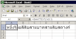
Introduction of BAHTTEXT function:

In Excel 2002, Microsoft introduced a new worksheet function: BAHTTEXT. This function converts a number to Thai text, and adds a suffix of "Baht." The figure below shows this function in action.

Now, I'm sure there are many people who welcome this new function. But here's why BAHTTEXT is listed in the "Oddities" section: Excel does not have a similar function to convert numbers to English text. In fact, BAHTTEXT is the only function that converts numbers to text.

A function to convert numbers to words is a common request in the Excel newsgroups. Yet, for some reason, Microsoft chose to use its development resources to create a BAHTTEXT function rather than a more generally useful NUMBERTEXT function.

So why did they choose Thai?

It's been suggested (by an anonymous Excel MVP) that the Excel programmers enjoy Thai food, and they created this function to facilitate email orders to Redmond Thai restaurants. This theory has not yet been confirmed -- but then again it hasn't been denied either.

Hijri Dates:

If you use the English language version of Excel 2002, try entering the text below into a cell:

A1-1

You'll get the result shown below! 

Furthermore, check the formula bar and you'll see that Excel interpreted your entry as a date -- March 25 of the current year. Take a look at the cell's number format, and you'll see that it's a custom format: B2d-mmm 

This same weirdness occurs with other text strings that begin with A1 followed by a hyphen. This, I've been told, is a Hijri (Islamic) date. But I haven't been told why a Hijri date pops up in an English language version of Excel.

If your company uses part numbers with this format, that's a good reason to avoid upgrading to Excel 2002.

Excel 11.0 (Excel 2003)

Only minor updates have been done in this version compared to Excel 2002. This version added additional support for XML. ‘Lists’ is another development worth noting. Information rights management was introduced where in you can specify who can read the document and who can edit it.

Microsoft is ending support for Excel 2003 on 8th April 2014.

We will continue to look about more recent versions of Excel in next post. Click here for next post.

Excel Versions: Excel 5.0 to 7.0

We started discussing about Excel 1.0 through Excel 4.0 in earlier post. Here is brief about Excel 5.0 to Excel 7.0

Excel 5.0

Released in 1993, Excel 5.0 was the first Excel version and office application to include Visual Basic for Applications (VBA), also called as Macro language. We will have series of posts on VBA in future but to touch base shortly, VBA is a programming language based on Visual Basic to add ability to automate tasks in excel and also create user defined functions. You can also record you actions that Excel saves as a code which can be used multiple times to automate simple tasks. However addition of VBA in Excel made it target for macro viruses. Antivirus applications started detecting these viruses and alerted users. Microsoft later came up with steps to prevent misuse by adding option to disable macros completely and enable trusted macros etc.

Excel 5.0 was the first spreadsheet to support multiple worksheets with in a single workbook.

Excel 5.0 contains an easter egg called ‘dot matrix credit display’. I don’t suppose anyone of us is using Excel 5.0 version now (Microsoft stopped support to this version very long back) but if you do have access to it, below are the steps to reach to the easter egg. 

1. Begin with a new (blank) worksheet displaying the standard toolbar. 
2. Right click on the toolbar. 
3. Choose CUSTOMIZE. 
4. Under CATAGORIES, scroll down to CUSTOM. 
5. Click and drag the solitaire (deck of cards) icon to the toolbar. 
6. When the ASSIGN MACRO box comes up, click OK. 
7. Close the CUSTOMIZE box. 
8. Press and hold CTRL-ALT-SHIFT, then left click on the solitaire icon. 

Excel 6.0

There was no version 6 of Excel. The version numbers jumped directly from 5 to 7 in order to bring all Office applications into a consistent version numbering system.

Excel 7.0 (Excel 95)

Excel 7.0 (Excel 95, we will use these two names interchangeably) was released with Windows 95 and as a part of Microsoft Office 95 version. This was the first time all major Office products like Word, Excel, PowerPoint has the same version number. This was the first version of Excel to use full 32-bit code. While this represented an improvement in the internal workings of Excel, it doesn't change the user's experience. Microsoft discontinued support for Office 95 programs in 2001/02.

Excel 7.0 has an impressive game (Easter egg) named 'Hall of Tortured Souls'. If you have access to excel 95, follow below steps to get to this game.Open Excel 95 with a blank work sheet 

1. Go down to the 95th row 
2. Select the whole row 
3. Tab over to column B 
4. Go to Help/About 
5. Hold down ctrl-alt-shift and click on the tech support button 
6. A window appears called 'Hall of Tortured Souls' 
7. At the end of the hall and all the programmers names do a 180 turn and type 'excelkfa' without quotes. 
8. Walk-through the wall and see the pictures.

We shall talk about next versions of Excel in later posts. Click here for Excel 8.0 to Excel 11.0.

Excel Versions : Excel 1.0 to 4.0

In this post, we will see a brief about MS Excel initial releases. This may help to know the history of Excel and how it came up as a market leader in its market.

Excel 1.0

Microsoft initial spreadsheet product was named as ‘Multiplan’ and was marketed in 1982. This was released for CP/M operating system (Control Program for Microcomputers released for Intel computers). Multiplan became very popular in CP/M OS but lost to its competitor Lotus 1-2-3 in MS-DOS platform. 

Microsoft released the first version of Excel (Excel 1.0) for Macintosh on September 30, 1985. Excel 1.0 was not released for Windows or MS-DOS. There never was a DOS version of Excel.

Excel 1.0 Screenshot

Excel 1.1

Excel 1.5

Excel 2.0

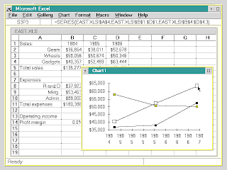
The first Windows version was labelled ‘Excel 2.0’ to correspond to the Mac version (Remember? Excel 1.0 was released only on Macintosh OS). First version of Excel released in 1987 for Windows 2.0 which completely outclassed the market leading Lotus123 spreadsheet both in terms of GUI and core functionality. Almost overnight Lotus started losing market share and within a few years it was no more than a memory. Lotus was the largest software company in the world and the spreadsheet was the most complex and profitable program around. Yet Microsoft steam-rolled right over it with the first release. Remarkable!

Excel 2.0 screenshot

Excel 2.1 Screenshot (notice grey borders and 3D)

Excel 2.2

Excel 2.2a

Excel 3.0

Excel 3.0 was released on 1990. It included toolbars, drawing capabilities, outlining, add-in support, 3D charts, and many more new features.

Excel 3.0 (First application to use a modern toolbar)

Excel 4.0

Released in 1992, Excel 4.0 introduced ‘Auto-fill’ feature for the first time.

Excel 4.0 had an easter egg (an intentional joke or hidden message in an application or program). It has a hidden animation of a dancing set of numbers 1 through 3, representing Lotus 1-2-3, which was then crushed by an Excel logo.

Continue to Excel 5.0 to 7.0 here.

A Brief History of Spreadsheet

The name Spread-sheet is used to represent ‘spread’ which is a paper that has two facing pages (think of centre page in a book or newspaper) and format used to present book-keeping ledgers—with columns for categories of expenditures across the top, invoices listed down the left margin, and the amount of each payment in the cell where its row and column intersect.

VisiCalc:

Developed by Dan Bricklin and Bob Frankston, VisiCalc is known as first electronic spreadsheet. This software was implemented in Apple II in 1979 and IBM PC in 1981. It has many features that modern day spreadsheet contain, for example: interactive user interface, automatic recalculation, status and formula lines, range copying with relative and absolute references, formula building by selecting referenced cells.

VisiCalc soon became so famous, people started buying PCs just to work on VisiCalc. Experts often attribute Apple II success with VisiCalc. 

Below is the screenshot of VisiCalc:

If you are enthusiastic on how it used to work, you can experience it by yourself by downloading a version of VisiCalc on your PC, it works on DOS. Here is the link to download and further information on this awesome age-old tool.

Lotus 1-2-3:

Late 1982, IBM introduced Lotus 1-2-3 specially for IBM PC. It started outselling VisiCalc soon after release and was in market as leader.

Microsoft Excel:

First developed on Macintosh platform, Excel was released first in 1985 and was quick to take over lion’s share of Lotus spreadsheet market. Since this is what this blog is created upon, we will see more on Excel in coming posts.

Quattro Pro, Gnumeric etc are other somewhat popular spreadsheets available.

Source: wikipedia.org

About Me

Hi There!!!!

Thanks for visiting my blog. 

I am Hari Krishna. I am a Chartered Accountant in service by profession. My attachment with Excel is about 10 years while I am writing this page. I was first introduced to Excel while I joined a CA firm as an Articled Assistant (part of CA course, never mind what it is!!) mostly to calculate tax liability and prepare audit reports etc. That was the first time I ever saw a spreadsheet. It quickly caught my awe. It was and has always been fun working with Excel. I soon started looking for new and easy ways to work on this platform and discovered that Excel is so much friendly once you tame it.

This blog is a way to share what I learnt in Excel over the years. For the record, I worked on Excel 95 (Version 7.0), 97 (V8.0), 2000 (V9.0), 2002 (V10.0), 2003 (V11.0), 2007 (V12.0), Excel 2010 (V14.0). and currently working on Excel 2013 (V15.0).

Looking back, I am so happy in transformation from being an occasional user of Excel to kind of expert (my friends and colleagues says so ;)) in advanced Excel and VBA. Down the line, I wrote many simple codes to ease routines and complex codes to achieve otherwise impossible or painstaking tasks in Excel.

I need not tell you guys how much Excel is used in offices for number crunching and analysis. I guess from a very small office employee to a decent corporate professional works largely on Excel. It’s real fun doing magic with keyboard short-cuts for repeated activities (imagine your colleagues saying OMG! what did you just do... when you use a short-cut with lightning fast), mastering the functions and to automate that boring day to day activities. I feel that with a bit of research and regular usage, anyone can become an expert in Excel.

I hope this blog will be useful in making your way to master Excel and get you appreciation from people around you. I welcome feedback on topics you want me to write on, report any errors in the article or a ‘thank you’ to keep me going. I will personally read all the comments and reply as soon as I can but please excuse me for little delay as I am working full time in a corporate and will not open blog / mails during office hours.

Here I conclude the introduction and wishing all the best. I hope you find what you came here for and happy learning. Cheerio.

Hari Krishna Popuri