Showing posts with label Tips & Tricks. Show all posts

Tuesday, March 25, 2014

Change Default File Format (.xlsx to .xls)


In my organisation, most of the people use Excel 2003 (you read it correct). I am one of the few privileged (canny??) to get Excel 2010 installed. So I got a version that is better in look and performance but a frequent problem I face is with the file formats. Any workbook I create in Excel 2010 will be by default contain extension “.xlsx” (recent file format). When I share these files with my colleagues, none of them will be able to modify that file in Excel 2003 and very few who is wise and installed compatibility pack will be able to read. I get a return mail saying they can’t open and I have to resave the file with “.xls” extension (Excel 2003 file format). I can do it for couple of files but if I have to do for every workbook, it would be good idea to change the default format to “.xls”. Let’s see how.

Excel 2010 and later:

File tab > Options > Save tab > Save workbooks segment > Select Excel 97-2003 Workbook in Save files in this format drop down > click OK.

Excel 2007:

Click the Microsoft Office button > Excel Options > Save tab > Save workbooks segment > Select Excel 97-2003 Workbook in Save files in this format drop down > click OK.


Convert Text Formatted Numbers to Actual Numbers


When I download reports from other programs such as SAP, often numbers are imported as text. Such numbers will be aligned left (common for actual text) and often indicated by error indicator (small green triangle on top left of those cells). These cells cannot be referenced in calculation formulas as Excel thinks it is actual text. Sometimes formatting the cells as Numbers works fine. Few times, it doesn't work. If I do F2 (edit the cell) and press Enter, then the cell value will be recognized as number. But doing this over thousands of cells manually will be irksome. If it sounds familiar to you, read on to see what we can do about it.

Excel 2002 and later versions are programmed to identify such cases and automatically convert these values to numbers. But if this hasn't happened by any reasons, we have few solutions below.

Solution 1: Try Formatting

Changing the format of the cells might work sometimes. So let’s try it. Click Home tab > Number group, select Number in the drop-down (in Excel 2007 or later) or Format menu > Cells > Number tab > under category, select Number (in Excel 2003 or earlier).

Does this solve the problem? If not, read on.

Solution 2: Use Error Checking

If those cells containing numbers as text are showing an error indicator, you may try this solution. Select all those cells. You will be able to see an error button (a square type of button with exclamation mark in it) next to the selection. Click on that and in the menu that appears, select Convert to Number.This action converts the numbers that are stored as text back to numbers.

Solution 3: Multiply by 1
  1. Select any empty cell anywhere
  2. Enter the value 1 into that cell
  3. Copy that cell (Ctrl+C)
  4. Select all the cells which needs to be converted
  5. Click Paste Special (one of the option in the right click menu)
  6. In the Paste Special dialogue box, select the Multiply option, then click OK.
This method forces a multiplication on the existing cells, while doing so Excel converts numbers in disguise to actual numbers.

Solution 4: Use TRIM function

Sometimes space before and after the actual number might cause Excel thinking that value is text. To clean up those spaces, use Excel’s built-in TRIM function.

Solution 5: Use SUBSTITUTE function

Some programs inserts spaces in between two digits in the same number (in one of the report I use, rupees and paise are separated by a space instead of dot). In this case, you can use SUBSTITUTE function to replace that space with a dot.

Solution 6: Use VALUE function

Value function converts any number, date or time formats entered as text to a number. Value function can also clean up the apostrophe normally entered in the start of the cell to show number as text.

Look at those numbers in disguise; they should be back as numbers by now.

Sunday, March 23, 2014

Insert Picture as Background in Comments


We insert comments to a cell for many reasons like to give additional information regarding the contents of the cell. But wherever I do that, I feel that Excel comment background is boring. I try to apply different backgrounds to see which one fits, in the process I discovered that you can also set a picture as a background to a comment. Interesting? Here is the way.

Once you are done inserting a comment, click on the border of it. Make sure you don’t have the cursor inside the comment. You can check that by the design across the borders. Comments outline appears like below when you are in edit comment mode or selection of comment.

When Comment is Selected

While Editing Comment

So diagonal lines indicates that you are in comment editing mode! Series of small dots is the proof that you just selected the comment. Right click on the dots part now and select Format Comment option. This should bring up Format Comment dialogue box; notice the tabs in this box, there should be more than 1 tab (if there is only Font tab, you might have right clicked in editing mode. So close the dialogue box and try again).

Click on Colors and Lines tab, in the color dropdown, select Fill Effects. In the new dialogue, click Picture tab and Select picture… button. Browse to your picture and select it. Click on Insert. Click OK in all the open boxes. You should be able to see selected picture in the comment background. (Look at the below pic, beautiful, isn't it? I selected blue hills which is available as a sample picture in MS Windows)

You can also change font, color, size, italic, bold and many other formatting optoins using Format Comment dialogue box.

Friday, March 21, 2014

Bored With Default Blue Colour??


Microsoft Office programs have a default colour scheme, Blue. Appearance of ribbons and menus will depend on this scheme. If you are bored with this colour, Office programs provide additional colours to play with. It’s often refreshing to see a different colour, you can check out below pictures to see how Excel looks under each colour.

Default Blue scheme

 Silver Scheme

Black Scheme

How to Change the Interface Colour Scheme

Excel 2007:

Click the Microsoft Office button > Excel Options > Popular tab > Top options for working with Excel segment > In Color Scheme drop down, select the colour you want from available options i.e. Blue, Silver & Blac.> click OK.

Excel 2010 and later:

File tab > Options > General > User Interface options segment > In Color Scheme drop down, select the colour you want from available options i.e. Blue, Silver & Black > click OK.

Excel 2003 menu colours depend on desktop theme. Read below to know how to change it.

How to Change the Windows Desktop Colour Scheme

Microsoft Windows theme determines the colour and appearance of Excel 2003 interface. Even in later versions of Excel, dialogue boxes use Windows theme settings. So even if you change interface colour scheme as above, you still have to match desktop colour scheme if you want a perfect sync look.

Right click in any empty space of desktop > Properties > Appearance tab > Under Windows and buttons, select Windows XP Style > Under Color Scheme drop down, select one of the available options i.e. Blue, Olive Green & Silver > click OK. Note that this will change the theme of desktop. You may also want to try other options available in these two drop down lists.

Note

Same Interface colour is used by all the Office programs (Except InfoPath 2007, OneNote 2007, Project 2007, Publisher 2007 and Visio 2007). Changing colour in one Office program will change the interface of all other Office programs.

The Mini Toolbar


Starting Excel 2007 for Windows, there is a cute mini tool bar introduced to quickly format your selection. You can see this tool bar by right clicking on any cell(s), shape or chart etc. It appears as below in my system when I right click on a cell.


Did you see on the top of right click menu? That’s the one I am talking about. If my Home tab is not displayed (where all formatting options are available  and I urgently want to apply quick formatting, mini tool bar is my friend.

Points to note:
  1. Contents of this menu depend on the object you right clicked. So, you will see a different menu if you click on a range and a different one if you click on chart etc.
  2. You cannot customize this menu based on your needs.
  3. Applies to Excel 2007 and later versions only (Not available in Mac 2008 & 2011)!
Though this is great to apply quick format, many users feel it annoying (I am not one of them). For those, you can turn this feature off. Let’s see how.

Excel 2007:

Click the Microsoft Office button > Excel Options > Popular tab > Top options for working with Excel segment > clear the Show Mini Toolbar on selection check box.

Excel 2010 and later:

File tab > Options > General > User Interface options segment > clear the Show Mini Toolbar on selection check box.

Show / Hide ScreenTips


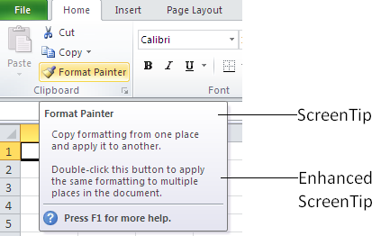
Did you notice the information window that appears when you place the mouse pointer on any of the command button or control? These small windows are called ScreenTips. More descriptive information on the button is called Enhanced ScreenTip. Below is the picture of Format Painter ScreenTip.


As a starter, this is a great feature to know which button is used for what. But as you know in and out of all the buttons, this may be a bit distractive at times. You can turn off this feature partly or fully (will explain) by following the procedure below.

Excel 2010 and later:

File tab > Options > General > User Interface options segment > In the ScreenTip style drop down, select the appropriate option
  • Show feature descriptions in ScreenTips: This option turns on ScreenTips and Enhanced ScreenTips. This is the default setting.
  • Don't show feature descriptions in ScreenTips: This option turns off Enhanced ScreenTips. You still see ScreenTips.
  • Don't show ScreenTips: This option turns off ScreenTips and Enhanced ScreenTips

Excel 2007:


Click the Microsoft Office button > Excel Options > Popular tab > Top options for working with Excel segment > In the ScreenTip style drop down, select the appropriate option (options are same as 2010 options, see above)

Excel 2003

Enhanced ScreenTips are not available in Excel 2003. Only ScreenTips are displayed, if you want to turn it off, below is the sequence.

Tools menu > Customize > Options tab > Under Other segment, select or clear the Show ScreenTips on toolbars checkbox.

Note:

Changing this setting effects all MS Office programs.

Debug Formulas Right in The Formula Bar


While you are creating complex formulas, it is often required to pause for a minute and see what is to come as a result of that formula. When you refer Sheet2!A1:A3 in a SUM function, It is often good idea to see what these cells A1:A3 contains and what is the result that SUM function fetches. Relevance of this becomes more when you build complex and sensitive formulas. Let’s see what Excel has to provide regarding this.

We have formula debugging tool in Excel that you can use to attain just the same. To simplify our example, I am going to use a simple SUM formula and show you what I mean.

Let’s assume I entered values 1, 2, 3 in cell A1, A2 and A3 respectively. I need to fetch sum of A1:A3 in cell A4.


We enter a formula in A4 which is “=SUM(A1:A3)”, after entering this formula, instead of pressing Enter, pause for a minute and notice the formula bar. Is it showing the formula you just entered? Click on the formula bar and select A1:A3 part.


Now press function key F9 and see what happens.


Saw the magic? Reference A1:A3 actually turned into the values that reference contains. If you want to show the entire formula result, you can press F9 without selecting any part of the formula.

Doing this action actually replaces the existing values with result. So, once you press F9 and are satisfied that displayed result is what you are expecting, press Ctrl+Z to undo your last action and restore the cell references. Otherwise, you can just press Enter if you don’t want formula anymore but only the result.

If you have made any error in cell reference or formula construction is incorrect, Excel throws up an error alert and you have to rectify the formula.

I deliberately gave incorrect reference as shown below and see the error.


This way you can use F9 in Formula bar as a calculator.

Let Excel Read Back What You Type


You can let the Excel talk to you by following below sequence. Excel’s text to speech conversion commands are “hidden” from normal user for the reason best known to Microsoft.

In Excel 2007 or later
  1. Next to the Quick Access Toolbar (on top of menu tab), click Customize Quick Access Toolbar (circled arrow below).
  2. Click More Commands.
  3. In the Choose commands from list, select All Commands.
  4. Scroll down, click the Speak Cells command, and then click Add. You can try out other options available too.
  5. Click OK.
  6. When you want to use a text-to-speech command, select the cells you want and click the button you added on the Quick Access Toolbar. (Keep speakers / headphones un-muted)
In Excel 2003 and 2002
  1. On the Tools menu, point to Speech, and then click Show Text to Speech Toolbar.
  2. On the Text To Speech toolbar, click the command that you want to use.

Format Numbers to Display Thousands / Millions


Sometimes you might want to display your numbers in multiples of thousands while retaining the actual values. For example: you have a number 10000 (ten thousand) in a cell. Keeping this, you want to show this number as 10. I do this all the time while presenting financial statements since numbers are huge. Do the following to achieve this.

Select the cell(s) you want to display in thousands, right click and select Format Cells. In the Format Cells dialogue box > Number tab > Select Custom in category > enter 0, (zero followed by a comma) in the Type box, click OK. Now see the cell value, it should have already become 10. Note that cell value 10000 is still there (you can notice in formula bar) but only displayed as 10 (in thousands)

Similarly, if you want in millions, Type box should contain 0,, (zero followed by two commas)

Tuesday, March 18, 2014

Combine Text and Formula In a Cell


We know how to enter values in cells. We also know how to enter formulas to play with numbers. But what if I have to combine text and formulas in one cell? For example: I want to show “Total bill value is 1000” where in 1000 comes from summing of cell A1:A10. So essentially we have to combine some text and a formula. Let’s see how to do it.

We will use Excel’s concatenation operator “&” and quotation marks to achieve this. In functions, text can be entered between two quotation marks. In the cell where you want the result, type the formula.
="Total bill value is " & SUM(A1:A10)
Easy? Yes it is.

I have another situation, I want to display “Today is DD:MMM:YYYY” wherein DD:MMM:YYYY is the date returned by Excel built-in function TODAY. How do I do it? I enter the below formula in any cell I want the result in.
="Today is " & TODAY()
That’s it? Actually no, if you tried entering this formula result will be something like this (on the day I am writing this post): Today is 41716. I wanted date but what is 41716? Actually this number is the date but since Excel considers entire cell to have text, you cannot format this number to date using Excel’s formatting options. You will have to do it in the function itself using another Excel built-in function TEXT. Let’s see the modified formula.
="Today is " & TEXT(TODAY(),"DD-MMM-YYYY")
This show up a result: Today is 18-Mar-2014. Just what I wanted! 

Enter Text Over Multiple Lines in a Cell

You can enter multiple lines of text in a cell by pressing Alt+Enter at the end of each line in the same cell. Excel automatically moves the cursor to one line below. Excel also automatically applies text wrapping to that cell.

One more thing that can help is, text entered this way can be easily copied and spread over multiple cells vertically in a way that each line occupies one cell. Try entering 3 lines (or any number you wish) of text with Alt+Enter at the end of every line and press Enter once done with all lines. Now select that cell again and press F2. Select all the text entered and copy it (Ctrl+c). Select any empty cell now and just paste (Ctrl+v). Your text will now occupy 3 cells, one for each line you entered.

Avoid Automatic Hyperlinks


When you type a value that resembles an email Id or a web address, Excel tries to be smart and formats the value to a hyper-link and change the font colour to blue with an underline. While most of the times this is pleasant, few times when I don’t want a hyper-link to be created or what I typed is just not a mail ID, this puts me off.

So, what options do we have?

Turn Off the Auto Formatting

If you don’t want Excel to format any value to hyper-link  you can just turn off this feature. Follow the steps below to do this.

In Excel 2010 or later

File Tab > Options > Proofing tab > AutoCorrect options > AutoFormat as you type tab > clear the check box below Replace as you type (i.e. next to Internet and network paths with hyperlinks).

Excel 2007

Click the Microsoft office button > Excel Options > Proofing tab > AutoCorrect options > AutoFormat as you type tab > clear the check box below Replace as you type (i.e. next to Internet and network paths with hyperlinks).

In Excel 2003 or earlier

Tools menu > AutoCorrect options > > AutoFormat as you type tab > clear the check box below Replace as you type (i.e. next to Internet and network paths with hyperlinks).

Follow the same steps but check this box if you want to enable this feature. This feature was introduced in Excel 2000 but there is no way to turn off this in that version. Above steps can be done only in Excel 2002 or later.

Override the Formatting

This is a quick workaround. Whenever Excel changes the format, just press Ctrl+Z (undo command). You will get the value you entered without hyper-link.

Enter Value with Apostrophe

You can start typing the text in to the cell with an apostrophe (‘). Then Excel treats this value as absolute text and will not try to include hyper-links.

Friday, March 14, 2014

Resize Scrollbars


Excel’s scrollbars size is not adjustable. By some reason if you want to increase or decrease these scrollbar size, your only hope is to change the scrollbar size settings at operating system level. Read on if you still want to go ahead as following steps will change scrollbar setting across all the programs.

This is the sequence in my Windows XP. Similar commands should be available in other OS as well.

Start > Control Panel > Appearance and Themes > Display (in category view)
Start > Control Panel > double click Display (in classic view)

In the Display Properties dialogue box, click on Appearance tab and click Advanced button! In Advanced Appearance dialogue box, under Item drop-down, select Scrollbar, adjust the size as per your needs to click OK in all open dialogue boxes.

Thursday, March 13, 2014

Fill Blank Cell with Non-Blank Cell Value Above


Assume a situation: I requested for spare parts available for many machines. My team had compiled that data from various sources and provided me as shown in below format.


Column B contains the part for each machine but what they did is machine number is entered in one cell only and its parts are spread in multiple cells in column B. Note that it’s data of thousands of machinery, I cannot really do any analysis on this data. For example: I cannot apply AutoFilter to see how many parts are available for a machine neither can I apply a pivot to summarize the data. In order to do that, I need to have the machine numbers against each part. How do you get this done?

Fortunately, we can do this very quickly in Excel. It only takes couple of seconds. Let’s see how.

Select all the cells of column A that has corresponding value in column B. Press Ctrl+G or F5. This opens up a dialogue box Go To. Click on Special in it, in the new box, check the radio button that reads Blanks and click OK. You should be able see all blank cells are selected as in below picture.


Now, start typing = and click on first non-blank cell above where = is placed and press Enter. In my example, when I type =, it automatically be placed in A3 and I click on cell A2 which is immediate non-blank cell above A3.


If I press Enter now, value in A2 will be placed in A3.


Now just press Ctrl+D or Home tab > Editing group > Fill > Down (Excel 2007 or later) or Edit menu > Fill > Down (Excel 2003 or earlier). This action should populate all the blank cells with immediate non-blank cells above.


One more (need based) step involves copying entire A column and paste as values in order to remove formulas. Now I can play with this data. Enjoy!

Work with Visible Cells Only

When you have few rows / columns hidden in between cells that you copy and paste, Excel copies and pastes contents of those cells which are hidden too. Or if you select any range and apply some formatting, Excel applies that formatting to hidden cells in that range as well. So what if you want to copy only visible cells or apply formatting to visible cells only?

Select the range you want, press Alt and ; (semicolon). This action selects only those cells which are visible. Copy and choose any place and paste it. Or apply any format you want and that will be applied only to visible cells.

Above method works. However there is another option if you want to simply copy and paste visible cells. Once you copy, paste this from Office Clipboard rather than using Enter or Ctrl+V

How to access Office Clipboard

To paste only visible cells, after you copy, select where you want to paste these values and follow the below steps.

Excel 2007 or later

Home tab > Clipboard group > click on the small arrow that is at the bottom right of this group. It will be under Format Painter option.Clicking this arrow opens up Clipboard. Locate your copied values and click on them with mouse.

Excel 2003 or earlier

Edit menu > Office Clipboard. Clicking this opens up Clipboard. Locate your copied values and click on them with mouse.

Note: Press Ctrl+C two times while copying will also opens up Office Clipboard under default conditions.

Wednesday, March 12, 2014

Few Little Known Paste Commands


When you copy any range, Excel comes up with variety of paste options. Most of these options are what we are already aware of like regular paste, paste only formulas, paste formats and combinations of these options. We also have few other options through paste special command.

There are few paste options we often don’t use or mostly overlook. Let’s see them now.

Paste as Link

If you are using Excel 2007 or later versions, this option links the range you copied by way of formulas in the sheet where you paste. Each cell in copied range will be referred by a formula from the pasted range.

Closest to this option in Excel 2003 is Paste as Hyperlink, but this option will only be activated if you copy content from any other program like Word, PowerPoint etc. This option creates a hyperlink to the file where you copied data from.

Paste as Picture

Whatever you copied will be pasted as a picture without any dependency on copied location anymore. You can use this picture just like any other picture you inserted from other locations.

Paste as Picture Link

This is my favourite option. You will have a picture of the copied data in all respects with one more awesome feature, that is the picture is linked to the source. If you change any value in the source data, this picture is automatically updated to reflect the change. That means Excel essentially creates a snapshot of copied range.

If you are using Excel 2007 or later versions, all the above commands can be found under Home tab > Clipboard group > Under the Paste drop-down.

In Excel 2003, Paste as Picture and Paste as Picture Link are available but hidden from normal eyes. You will have to keep pressing Shift key while clicking Edit menu to see these commands. 

Do Basic Math Operations by Paste Special


I have to submit most of the reports for financial statements in millions of dollars ($ ML) denomination. But data output from my accounting software comes along with its decimal values too. How do I quickly convert this into millions?

Normally most of the people I saw will insert a column next to the output values column and enter a formula “=Output value cell address /1000000” (of course, you have to replace the name in formula with actual references). This method is fine if you want to show the initial values too. But my stakeholders are not interested in seeing that. So, I have to copy the converted values and paste there again as values using paste special.

There is an alternate and quick way, you can use Paste Special functionality in this case. Just enter “1000000” in any of the empty cell. Copy it and now select all your data output values. Right click, select Paste Special. Under Operation segment, click on Divide. That’s it, you have just converted all the output values into millions.

If you notice, there are other operators also in Paste Special to perform addition, subtraction & multiplication along with division. Go ahead and use them extensively. Enjoy!!

Hide Content of the Cells


We have discussed this method in a previous post on Excel protection features.

Suppose you are sending a file to a friend and do not want him/her to see what a particular cell contains. Then you simply format the cell to make contents of it invisible on its face.

Select the cell(s) you want and press Ctrl+1 (or simply right click and select Format cells option). In the Number tab, under Category, select Custom and under Type, enter ;;; (3 semicolons without spaces) and hit OK. Contents of selected cells will not be visible any more in the cell. However you can still see them in formula bar. This option is best used in conditional formatting to highlight cell colours but not contents.

Note that this option only make the content of the cell invisible but will not delete it. You can use the content just the way you do with any other cell in formulas etc.

You may also wish to see how to hide contents of the cell in formula bar.

Hide Formulas & Contents in Formula Bar


Many a times, I create complex formulas and I don’t normally want my novice users to see them. That’s may be because I am afraid that they may mess up those formulas or I just want to keep the recipe of the formulas to myself (secret?). Whatever is the reason, this is what I do in that case.

If you read our Excel’s protection features post, you are already aware of what I am going to say below.

Every cell has two key properties: locked and hidden. A locked cell can't be changed, and the contents of a hidden cell don't appear in the formula bar when the cell is selected. By default, every cell is locked and not hidden. But it's important to remember that these attributes have no effect unless the worksheet itself is protected.

Select the cells where formulas / contents to be hidden in formula bar. In the Format cells dialogue box (Ctrl+1), under Protection tab, make sure check box Hidden is checked and click OK. Then go to Tools > Protection > Protect Sheet and hit OK (In Excel 2003) or Review > Protect Sheet and hit OK (Excel 2007 and later).

This makes the result of the formula visible in the cell and formulas itself are not visible in formula bar. Users can un-protect the sheet and see the content in formula bar. You can use this feature to hide contents of the cells too in formula bar.

If you don’t want user to un-protect without a password, you can password protect these sheets. You can read more on the protection features here.

Tuesday, March 11, 2014

Get Rid of That Annoying Update Links Alert


Hello!! Are you familiar with that annoying alert Excel pops up when you open a workbook? Around half of the workbooks I receive over emails shows me this alert. A screenshot of this error is given below.


If you also get this alert and want to get rid of it, read on.

This alert is often caused by broken links that your formulas refer to. But that may not be the only case. Let’s see the various reasons and what to do.

Most probable cause might be your formulas. Check all the formulas in your workbook by pressing Ctrl+` (we already discussed about this in a previous post). If there is any formula that is referring to external workbook or showing a #REF! error, edit the formula.

Click on Edit Links… button in the alert or you can access it by Data tab > Connections group > Edit Links (Excel 2007 or later) or Edit menu > Links (In Excel 2003 or earlier). Any of this action opens a dialogue box Edit Links which looks like as in below picture. (I hid the actual source, confidential!!)


If you have any workbook name appearing under Source, that might be the culprit. You can choose from various options in this dialogue box to update values from Source book or change Source or open the source to make sure it is available or break the link. Status column under source will show you if that source is causing error or not. You can refresh the source status by clicking on Check Status. There is a button available at the left bottom to set an option for start-up prompt.


These options are self-explanatory. You can ask Excel to sit silent even if the links are broken by selecting one of Don’t display alert ….. options!

If this does not solve your problem, there might be another cause. Open Name Manager in that workbook (read this post to know more about Named Ranges) and see Refers To: field for all the names. If a name refers to another workbook or it contains an error like !#REF! then edit the names or delete them if they are not required. This is one of the common causes for broken links.

No luck yet? No worries. Check if you have charts in that workbook. If you do, click on each data series and see if the series formula refers to within the workbook. If this formula refers to external workbook, copy that data to current workbook and edit / delete the existing link.

Save your workbook and reopen it. Now your workbook should open without this alert. Happy?